Extended Common Load Modelling : example
Import the required modules
[1]:
%matplotlib inline
import openturns as ot
import oteclm
from openturns.viewer import View
We consider a common cause failure (CCF) groupe with n=7 identical and independent components. The total impact vector of this CCF group is estimated after N=1002100 demands or tests on the group.
![V_t^{n,N} = [1000000, 2000, 200, 30, 20, 5, 0, 0]](data:image/svg+xml;base64,PD94bWwgdmVyc2lvbj0nMS4wJyBlbmNvZGluZz0nVVRGLTgnPz4KPCEtLSBUaGlzIGZpbGUgd2FzIGdlbmVyYXRlZCBieSBkdmlzdmdtIDIuOC4xIC0tPgo8c3ZnIHZlcnNpb249JzEuMScgeG1sbnM9J2h0dHA6Ly93d3cudzMub3JnLzIwMDAvc3ZnJyB4bWxuczp4bGluaz0naHR0cDovL3d3dy53My5vcmcvMTk5OS94bGluaycgd2lkdGg9JzIwNi44NTYxODJwdCcgaGVpZ2h0PScxNC4xMDI2NDhwdCcgdmlld0JveD0nOTAuODQzMzg5IC0xNS4yOTgyMDcgMjA2Ljg1NjE4MiAxNC4xMDI2NDgnPgo8ZGVmcz4KPHBhdGggaWQ9J2cyLTQ4JyBkPSdNNS4zNTU5MTUtMy44MjU2NTRDNS4zNTU5MTUtNC44MTc5MzMgNS4yOTYxMzktNS43ODYzMDEgNC44NjU3NTMtNi42OTQ4OTRDNC4zNzU1OTItNy42ODcxNzMgMy41MTQ4MTktNy45NTAxODcgMi45MjkwMTYtNy45NTAxODdDMi4yMzU2MTYtNy45NTAxODcgMS4zODY4LTcuNjAzNDg3IC45NDQ0NTgtNi42MTEyMDhDLjYwOTcxNC01Ljg1ODAzMiAuNDkwMTYyLTUuMTE2ODEyIC40OTAxNjItMy44MjU2NTRDLjQ5MDE2Mi0yLjY2NjAwMiAuNTczODQ4LTEuNzkzMjc1IDEuMDA0MjM0LS45NDQ0NThDMS40NzA0ODYtLjAzNTg2NiAyLjI5NTM5MiAuMjUxMDU5IDIuOTE3MDYxIC4yNTEwNTlDMy45NTcxNjEgLjI1MTA1OSA0LjU1NDkxOS0uMzcwNjEgNC45MDE2MTktMS4wNjQwMUM1LjMzMjAwNS0xLjk2MDY0OCA1LjM1NTkxNS0zLjEzMjI1NCA1LjM1NTkxNS0zLjgyNTY1NFpNMi45MTcwNjEgLjAxMTk1NUMyLjUzNDQ5NiAuMDExOTU1IDEuNzU3NDEtLjIwMzIzOCAxLjUzMDI2Mi0xLjUwNjM1MUMxLjM5ODc1NS0yLjIyMzY2MSAxLjM5ODc1NS0zLjEzMjI1NCAxLjM5ODc1NS0zLjk2OTExNkMxLjM5ODc1NS00Ljk0OTQ0IDEuMzk4NzU1LTUuODM0MTIyIDEuNTkwMDM3LTYuNTM5NDc3QzEuNzkzMjc1LTcuMzQwNDczIDIuNDAyOTg5LTcuNzExMDgzIDIuOTE3MDYxLTcuNzExMDgzQzMuMzcxMzU3LTcuNzExMDgzIDQuMDY0NzU3LTcuNDM2MTE1IDQuMjkxOTA1LTYuNDA3OTdDNC40NDczMjMtNS43MjY1MjYgNC40NDczMjMtNC43ODIwNjcgNC40NDczMjMtMy45NjkxMTZDNC40NDczMjMtMy4xNjgxMiA0LjQ0NzMyMy0yLjI1OTUyNyA0LjMxNTgxNi0xLjUzMDI2MkM0LjA4ODY2Ny0uMjE1MTkzIDMuMzM1NDkyIC4wMTE5NTUgMi45MTcwNjEgLjAxMTk1NVonLz4KPHBhdGggaWQ9J2cyLTQ5JyBkPSdNMy40NDMwODgtNy42NjMyNjNDMy40NDMwODgtNy45MzgyMzIgMy40NDMwODgtNy45NTAxODcgMy4yMDM5ODUtNy45NTAxODdDMi45MTcwNjEtNy42MjczOTcgMi4zMTkzMDMtNy4xODUwNTYgMS4wODc5Mi03LjE4NTA1NlYtNi44MzgzNTZDMS4zNjI4ODktNi44MzgzNTYgMS45NjA2NDgtNi44MzgzNTYgMi42MTgxODItNy4xNDkxOTFWLS45MjA1NDhDMi42MTgxODItLjQ5MDE2MiAyLjU4MjMxNi0uMzQ2NyAxLjUzMDI2Mi0uMzQ2N0gxLjE1OTY1MVYwQzEuNDgyNDQxLS4wMjM5MSAyLjY0MjA5Mi0uMDIzOTEgMy4wMzY2MTMtLjAyMzkxUzQuNTc4ODI5LS4wMjM5MSA0LjkwMTYxOSAwVi0uMzQ2N0g0LjUzMTAwOUMzLjQ3ODk1NC0uMzQ2NyAzLjQ0MzA4OC0uNDkwMTYyIDMuNDQzMDg4LS45MjA1NDhWLTcuNjYzMjYzWicvPgo8cGF0aCBpZD0nZzItNTAnIGQ9J001LjI2MDI3NC0yLjAwODQ2OEg0Ljk5NzI2QzQuOTYxMzk1LTEuODA1MjMgNC44NjU3NTMtMS4xNDc2OTYgNC43NDYyMDItLjk1NjQxM0M0LjY2MjUxNi0uODQ4ODE3IDMuOTgxMDcxLS44NDg4MTcgMy42MjI0MTYtLjg0ODgxN0gxLjQxMDcxQzEuNzMzNDk5LTEuMTIzNzg2IDIuNDYyNzY1LTEuODg4OTE3IDIuNzczNTk5LTIuMTc1ODQxQzQuNTkwNzg1LTMuODQ5NTY0IDUuMjYwMjc0LTQuNDcxMjMzIDUuMjYwMjc0LTUuNjU0Nzk1QzUuMjYwMjc0LTcuMDI5NjM5IDQuMTcyMzU0LTcuOTUwMTg3IDIuNzg1NTU0LTcuOTUwMTg3Uy41ODU4MDMtNi43NjY2MjUgLjU4NTgwMy01LjczODQ4MUMuNTg1ODAzLTUuMTI4NzY3IDEuMTExODMxLTUuMTI4NzY3IDEuMTQ3Njk2LTUuMTI4NzY3QzEuMzk4NzU1LTUuMTI4NzY3IDEuNzA5NTg5LTUuMzA4MDk1IDEuNzA5NTg5LTUuNjkwNjZDMS43MDk1ODktNi4wMjU0MDUgMS40ODI0NDEtNi4yNTI1NTMgMS4xNDc2OTYtNi4yNTI1NTNDMS4wNDAxLTYuMjUyNTUzIDEuMDE2MTg5LTYuMjUyNTUzIC45ODAzMjQtNi4yNDA1OThDMS4yMDc0NzItNy4wNTM1NDkgMS44NTMwNTEtNy42MDM0ODcgMi42MzAxMzctNy42MDM0ODdDMy42NDYzMjYtNy42MDM0ODcgNC4yNjc5OTUtNi43NTQ2NyA0LjI2Nzk5NS01LjY1NDc5NUM0LjI2Nzk5NS00LjYzODYwNSAzLjY4MjE5Mi0zLjc1MzkyMyAzLjAwMDc0Ny0yLjk4ODc5MkwuNTg1ODAzLS4yODY5MjRWMEg0Ljk0OTQ0TDUuMjYwMjc0LTIuMDA4NDY4WicvPgo8cGF0aCBpZD0nZzItNTEnIGQ9J00yLjE5OTc1MS00LjI5MTkwNUMxLjk5NjUxMy00LjI3OTk1IDEuOTQ4NjkyLTQuMjY3OTk1IDEuOTQ4NjkyLTQuMTYwMzk5QzEuOTQ4NjkyLTQuMDQwODQ3IDIuMDA4NDY4LTQuMDQwODQ3IDIuMjIzNjYxLTQuMDQwODQ3SDIuNzczNTk5QzMuNzg5Nzg4LTQuMDQwODQ3IDQuMjQ0MDg1LTMuMjAzOTg1IDQuMjQ0MDg1LTIuMDU2Mjg5QzQuMjQ0MDg1LS40OTAxNjIgMy40MzExMzMtLjA3MTczMSAyLjg0NTMzLS4wNzE3MzFDMi4yNzE0ODItLjA3MTczMSAxLjI5MTE1OC0uMzQ2NyAuOTQ0NDU4LTEuMTM1NzQxQzEuMzI3MDI0LTEuMDc1OTY1IDEuNjczNzI0LTEuMjkxMTU4IDEuNjczNzI0LTEuNzIxNTQ0QzEuNjczNzI0LTIuMDY4MjQ0IDEuNDIyNjY1LTIuMzA3MzQ3IDEuMDg3OTItMi4zMDczNDdDLjgwMDk5Ni0yLjMwNzM0NyAuNDkwMTYyLTIuMTM5OTc1IC40OTAxNjItMS42ODU2NzlDLjQ5MDE2Mi0uNjIxNjY5IDEuNTU0MTcyIC4yNTEwNTkgMi44ODExOTYgLjI1MTA1OUM0LjMwMzg2MSAuMjUxMDU5IDUuMzU1OTE1LS44MzY4NjIgNS4zNTU5MTUtMi4wNDQzMzRDNS4zNTU5MTUtMy4xNDQyMDkgNC40NzEyMzMtNC4wMDQ5ODEgMy4zMjM1MzctNC4yMDgyMTlDNC4zNjM2MzYtNC41MDcwOTggNS4wMzMxMjYtNS4zNzk4MjYgNS4wMzMxMjYtNi4zMTIzMjlDNS4wMzMxMjYtNy4yNTY3ODcgNC4wNTI4MDItNy45NTAxODcgMi44OTMxNTEtNy45NTAxODdDMS42OTc2MzQtNy45NTAxODcgLjgxMjk1MS03LjIyMDkyMiAuODEyOTUxLTYuMzQ4MTk0Qy44MTI5NTEtNS44Njk5ODggMS4xODM1NjItNS43NzQzNDYgMS4zNjI4ODktNS43NzQzNDZDMS42MTM5NDgtNS43NzQzNDYgMS45MDA4NzItNS45NTM2NzQgMS45MDA4NzItNi4zMTIzMjlDMS45MDA4NzItNi42OTQ4OTQgMS42MTM5NDgtNi44NjIyNjcgMS4zNTA5MzQtNi44NjIyNjdDMS4yNzkyMDMtNi44NjIyNjcgMS4yNTUyOTMtNi44NjIyNjcgMS4yMTk0MjctNi44NTAzMTFDMS42NzM3MjQtNy42NjMyNjMgMi43OTc1MDktNy42NjMyNjMgMi44NTcyODUtNy42NjMyNjNDMy4yNTE4MDYtNy42NjMyNjMgNC4wMjg4OTItNy40ODM5MzUgNC4wMjg4OTItNi4zMTIzMjlDNC4wMjg4OTItNi4wODUxODEgMy45OTMwMjYtNS40MTU2OTEgMy42NDYzMjYtNC45MDE2MTlDMy4yODc2NzEtNC4zNzU1OTIgMi44ODExOTYtNC4zMzk3MjYgMi41NTg0MDYtNC4zMjc3NzFMMi4xOTk3NTEtNC4yOTE5MDVaJy8+CjxwYXRoIGlkPSdnMi01MycgZD0nTTEuNTMwMjYyLTYuODUwMzExQzIuMDQ0MzM0LTYuNjgyOTM5IDIuNDYyNzY1LTYuNjcwOTg0IDIuNTk0MjcxLTYuNjcwOTg0QzMuOTQ1MjA1LTYuNjcwOTg0IDQuODA1OTc4LTcuNjYzMjYzIDQuODA1OTc4LTcuODMwNjM1QzQuODA1OTc4LTcuODc4NDU2IDQuNzgyMDY3LTcuOTM4MjMyIDQuNzEwMzM2LTcuOTM4MjMyQzQuNjg2NDI2LTcuOTM4MjMyIDQuNjYyNTE2LTcuOTM4MjMyIDQuNTU0OTE5LTcuODkwNDExQzMuODg1NDMtNy42MDM0ODcgMy4zMTE1ODItNy41Njc2MjEgMy4wMDA3NDctNy41Njc2MjFDMi4yMTE3MDYtNy41Njc2MjEgMS42NDk4MTMtNy44MDY3MjUgMS40MjI2NjUtNy45MDIzNjZDMS4zMzg5NzktNy45MzgyMzIgMS4zMTUwNjgtNy45MzgyMzIgMS4zMDMxMTMtNy45MzgyMzJDMS4yMDc0NzItNy45MzgyMzIgMS4yMDc0NzItNy44NjY1MDEgMS4yMDc0NzItNy42NzUyMThWLTQuMTI0NTMzQzEuMjA3NDcyLTMuOTA5MzQgMS4yMDc0NzItMy44Mzc2MDkgMS4zNTA5MzQtMy44Mzc2MDlDMS40MTA3MS0zLjgzNzYwOSAxLjQyMjY2NS0zLjg0OTU2NCAxLjU0MjIxNy0zLjk5MzAyNkMxLjg3Njk2MS00LjQ4MzE4OCAyLjQzODg1NC00Ljc3MDExMiAzLjAzNjYxMy00Ljc3MDExMkMzLjY3MDIzNy00Ljc3MDExMiAzLjk4MTA3MS00LjE4NDMwOSA0LjA3NjcxMi0zLjk4MTA3MUM0LjI3OTk1LTMuNTE0ODE5IDQuMjkxOTA1LTIuOTI5MDE2IDQuMjkxOTA1LTIuNDc0NzJTNC4yOTE5MDUtMS4zMzg5NzkgMy45NTcxNjEtLjgwMDk5NkMzLjY5NDE0Ny0uMzcwNjEgMy4yMjc4OTUtLjA3MTczMSAyLjcwMTg2OC0uMDcxNzMxQzEuOTEyODI3LS4wNzE3MzEgMS4xMzU3NDEtLjYwOTcxNCAuOTIwNTQ4LTEuNDgyNDQxQy45ODAzMjQtMS40NTg1MzEgMS4wNTIwNTUtMS40NDY1NzUgMS4xMTE4MzEtMS40NDY1NzVDMS4zMTUwNjgtMS40NDY1NzUgMS42Mzc4NTgtMS41NjYxMjcgMS42Mzc4NTgtMS45NzI2MDNDMS42Mzc4NTgtMi4zMDczNDcgMS40MTA3MS0yLjQ5ODYzIDEuMTExODMxLTIuNDk4NjNDLjg5NjYzOC0yLjQ5ODYzIC41ODU4MDMtMi4zOTEwMzQgLjU4NTgwMy0xLjkyNDc4MkMuNTg1ODAzLS45MDg1OTMgMS4zOTg3NTUgLjI1MTA1OSAyLjcyNTc3OCAuMjUxMDU5QzQuMDc2NzEyIC4yNTEwNTkgNS4yNjAyNzQtLjg4NDY4MiA1LjI2MDI3NC0yLjQwMjk4OUM1LjI2MDI3NC0zLjgyNTY1NCA0LjMwMzg2MS01LjAwOTIxNSAzLjA0ODU2OC01LjAwOTIxNUMyLjM2NzEyMy01LjAwOTIxNSAxLjg0MTA5Ni00LjcxMDMzNiAxLjUzMDI2Mi00LjM3NTU5MlYtNi44NTAzMTFaJy8+CjxwYXRoIGlkPSdnMi02MScgZD0nTTguMDY5NzM4LTMuODczNDc0QzguMjM3MTExLTMuODczNDc0IDguNDUyMzA0LTMuODczNDc0IDguNDUyMzA0LTQuMDg4NjY3QzguNDUyMzA0LTQuMzE1ODE2IDguMjQ5MDY2LTQuMzE1ODE2IDguMDY5NzM4LTQuMzE1ODE2SDEuMDI4MTQ0Qy44NjA3NzItNC4zMTU4MTYgLjY0NTU3OS00LjMxNTgxNiAuNjQ1NTc5LTQuMTAwNjIzQy42NDU1NzktMy44NzM0NzQgLjg0ODgxNy0zLjg3MzQ3NCAxLjAyODE0NC0zLjg3MzQ3NEg4LjA2OTczOFpNOC4wNjk3MzgtMS42NDk4MTNDOC4yMzcxMTEtMS42NDk4MTMgOC40NTIzMDQtMS42NDk4MTMgOC40NTIzMDQtMS44NjUwMDZDOC40NTIzMDQtMi4wOTIxNTQgOC4yNDkwNjYtMi4wOTIxNTQgOC4wNjk3MzgtMi4wOTIxNTRIMS4wMjgxNDRDLjg2MDc3Mi0yLjA5MjE1NCAuNjQ1NTc5LTIuMDkyMTU0IC42NDU1NzktMS44NzY5NjFDLjY0NTU3OS0xLjY0OTgxMyAuODQ4ODE3LTEuNjQ5ODEzIDEuMDI4MTQ0LTEuNjQ5ODEzSDguMDY5NzM4WicvPgo8cGF0aCBpZD0nZzItOTEnIGQ9J00yLjk4ODc5MiAyLjk4ODc5MlYyLjU0NjQ1MUgxLjgyOTE0MVYtOC41MjQwMzVIMi45ODg3OTJWLTguOTY2Mzc2SDEuMzg2OFYyLjk4ODc5MkgyLjk4ODc5MlonLz4KPHBhdGggaWQ9J2cyLTkzJyBkPSdNMS44NTMwNTEtOC45NjYzNzZILjI1MTA1OVYtOC41MjQwMzVIMS40MTA3MVYyLjU0NjQ1MUguMjUxMDU5VjIuOTg4NzkySDEuODUzMDUxVi04Ljk2NjM3NlonLz4KPHBhdGggaWQ9J2cwLTU5JyBkPSdNMS40OTA0MTEtLjExOTU1MkMxLjQ5MDQxMSAuMzk4NTA2IDEuMzc4ODI5IC44NTI4MDIgLjg4NDY4MiAxLjM0Njk0OUMuODUyODAyIDEuMzcwODU5IC44MzY4NjIgMS4zODY4IC44MzY4NjIgMS40MjY2NUMuODM2ODYyIDEuNDkwNDExIC45MDA2MjMgMS41MzgyMzIgLjk1NjQxMyAxLjUzODIzMkMxLjA1MjA1NSAxLjUzODIzMiAxLjcxMzU3NCAuOTA4NTkzIDEuNzEzNTc0LS4wMjM5MUMxLjcxMzU3NC0uNTMzOTk4IDEuNTIyMjkxLS44ODQ2ODIgMS4xNzE2MDYtLjg4NDY4MkMuODkyNjUzLS44ODQ2ODIgLjczMzI1LS42NjE1MTkgLjczMzI1LS40NDYzMjZDLjczMzI1LS4yMjMxNjMgLjg4NDY4MiAwIDEuMTc5NTc3IDBDMS4zNzA4NTkgMCAxLjQ5MDQxMS0uMTExNTgyIDEuNDkwNDExLS4xMTk1NTJaJy8+CjxwYXRoIGlkPSdnMC03OCcgZD0nTTYuMzEyMzI5LTQuNTc0ODQ0QzYuNDA3OTctNC45NjUzOCA2LjU4MzMxMy01LjE1NjY2MyA3LjE1NzE2MS01LjE4MDU3M0M3LjIzNjg2Mi01LjE4MDU3MyA3LjMwMDYyMy01LjIyODM5NCA3LjMwMDYyMy01LjMzMjAwNUM3LjMwMDYyMy01LjM3OTgyNiA3LjI2MDc3Mi01LjQ0MzU4NyA3LjE4MTA3MS01LjQ0MzU4N0M3LjEyNTI4LTUuNDQzNTg3IDYuOTczODQ4LTUuNDE5Njc2IDYuMzg0MDYtNS40MTk2NzZDNS43NDY0NTEtNS40MTk2NzYgNS42NDI4MzktNS40NDM1ODcgNS41NzExMDgtNS40NDM1ODdDNS40NDM1ODctNS40NDM1ODcgNS40MTk2NzYtNS4zNTU5MTUgNS40MTk2NzYtNS4yOTIxNTRDNS40MTk2NzYtNS4xODg1NDMgNS41MjMyODgtNS4xODA1NzMgNS41OTUwMTktNS4xODA1NzNDNi4wODExOTYtNS4xNjQ2MzMgNi4wODExOTYtNC45NDk0NCA2LjA4MTE5Ni00LjgzNzg1OEM2LjA4MTE5Ni00Ljc5ODAwNyA2LjA4MTE5Ni00Ljc1ODE1NyA2LjA0OTMxNS00LjYzMDYzNUw1LjE3MjYwMy0xLjEzOTcyNkwzLjI1MTgwNi01LjMwMDEyNUMzLjE4ODA0NS01LjQ0MzU4NyAzLjE3MjEwNS01LjQ0MzU4NyAyLjk4MDgyMi01LjQ0MzU4N0gxLjk0NDcwN0MxLjgwMTI0NS01LjQ0MzU4NyAxLjY5NzYzNC01LjQ0MzU4NyAxLjY5NzYzNC01LjI5MjE1NEMxLjY5NzYzNC01LjE4MDU3MyAxLjc5MzI3NS01LjE4MDU3MyAxLjk2MDY0OC01LjE4MDU3M0MyLjAyNDQwOC01LjE4MDU3MyAyLjI2MzUxMi01LjE4MDU3MyAyLjQ0NjgyNC01LjEzMjc1MkwxLjM3ODgyOS0uODUyODAyQzEuMjgzMTg4LS40NTQyOTYgMS4wNzU5NjUtLjI3ODk1NCAuNTQxOTY4LS4yNjMwMTRDLjQ5NDE0Ny0uMjYzMDE0IC4zOTg1MDYtLjI1NTA0NCAuMzk4NTA2LS4xMTE1ODJDLjM5ODUwNi0uMDYzNzYxIC40MzgzNTYgMCAuNTE4MDU3IDBDLjU0OTkzOCAwIC43MzMyNS0uMDIzOTEgMS4zMDcwOTgtLjAyMzkxQzEuOTM2NzM3LS4wMjM5MSAyLjA1NjI4OSAwIDIuMTI4MDIgMEMyLjE1OTkgMCAyLjI3OTQ1MiAwIDIuMjc5NDUyLS4xNTE0MzJDMi4yNzk0NTItLjI0NzA3MyAyLjE5MTc4MS0uMjYzMDE0IDIuMTM1OTktLjI2MzAxNEMxLjg0OTA2Ni0uMjcwOTg0IDEuNjA5OTYzLS4zMTg4MDQgMS42MDk5NjMtLjU5Nzc1OEMxLjYwOTk2My0uNjM3NjA5IDEuNjMzODczLS43NDkxOTEgMS42MzM4NzMtLjc1NzE2MUwyLjY3Nzk1OC00LjkxNzU1OUgyLjY4NTkyOEw0LjkwMTYxOS0uMTQzNDYyQzQuOTU3NDEtLjAxNTk0IDQuOTY1MzggMCA1LjA1MzA1MSAwQzUuMTY0NjMzIDAgNS4xNzI2MDMtLjAzMTg4IDUuMjA0NDgzLS4xNjczNzJMNi4zMTIzMjktNC41NzQ4NDRaJy8+CjxwYXRoIGlkPSdnMC0xMTAnIGQ9J00xLjU5NDAyMi0xLjMwNzA5OEMxLjYxNzkzMy0xLjQyNjY1IDEuNjk3NjM0LTEuNzI5NTE0IDEuNzIxNTQ0LTEuODQ5MDY2QzEuODMzMTI2LTIuMjc5NDUyIDEuODMzMTI2LTIuMjg3NDIyIDIuMDE2NDM4LTIuNTUwNDM2QzIuMjc5NDUyLTIuOTQwOTcxIDIuNjU0MDQ3LTMuMjkxNjU2IDMuMTg4MDQ1LTMuMjkxNjU2QzMuNDc0OTY5LTMuMjkxNjU2IDMuNjQyMzQxLTMuMTI0Mjg0IDMuNjQyMzQxLTIuNzQ5Njg5QzMuNjQyMzQxLTIuMzExMzMzIDMuMzA3NTk3LTEuNDAyNzQgMy4xNTYxNjQtMS4wMTIyMDRDMy4wNTI1NTMtLjc0OTE5MSAzLjA1MjU1My0uNzAxMzcgMy4wNTI1NTMtLjU5Nzc1OEMzLjA1MjU1My0uMTQzNDYyIDMuNDI3MTQ4IC4wNzk3MDEgMy43Njk4NjMgLjA3OTcwMUM0LjU1MDkzNCAuMDc5NzAxIDQuODc3NzA5LTEuMDM2MTE1IDQuODc3NzA5LTEuMTM5NzI2QzQuODc3NzA5LTEuMjE5NDI3IDQuODEzOTQ4LTEuMjQzMzM3IDQuNzU4MTU3LTEuMjQzMzM3QzQuNjYyNTE2LTEuMjQzMzM3IDQuNjQ2NTc1LTEuMTg3NTQ3IDQuNjIyNjY1LTEuMTA3ODQ2QzQuNDMxMzgyLS40NTQyOTYgNC4wOTY2MzgtLjE0MzQ2MiAzLjc5Mzc3My0uMTQzNDYyQzMuNjY2MjUyLS4xNDM0NjIgMy42MDI0OTEtLjIyMzE2MyAzLjYwMjQ5MS0uNDA2NDc2UzMuNjY2MjUyLS43NjUxMzEgMy43NDU5NTMtLjk2NDM4NEMzLjg2NTUwNC0xLjI2NzI0OCA0LjIxNjE4OS0yLjE4MzgxMSA0LjIxNjE4OS0yLjYzMDEzN0M0LjIxNjE4OS0zLjIyNzg5NSAzLjgwMTc0My0zLjUxNDgxOSAzLjIyNzg5NS0zLjUxNDgxOUMyLjU4MjMxNi0zLjUxNDgxOSAyLjE2Nzg3LTMuMTI0Mjg0IDEuOTM2NzM3LTIuODIxNDJDMS44ODA5NDYtMy4yNTk3NzYgMS41MzAyNjItMy41MTQ4MTkgMS4xMjM3ODYtMy41MTQ4MTlDLjgzNjg2Mi0zLjUxNDgxOSAuNjM3NjA5LTMuMzMxNTA3IC41MTAwODctMy4wODQ0MzNDLjMxODgwNC0yLjcwOTgzOCAuMjM5MTAzLTIuMzExMzMzIC4yMzkxMDMtMi4yOTUzOTJDLjIzOTEwMy0yLjIyMzY2MSAuMjk0ODk0LTIuMTkxNzgxIC4zNTg2NTUtMi4xOTE3ODFDLjQ2MjI2Ny0yLjE5MTc4MSAuNDcwMjM3LTIuMjIzNjYxIC41MjYwMjctMi40MzA4ODRDLjYyMTY2OS0yLjgyMTQyIC43NjUxMzEtMy4yOTE2NTYgMS4wOTk4NzUtMy4yOTE2NTZDMS4zMDcwOTgtMy4yOTE2NTYgMS4zNTQ5MTktMy4wOTI0MDMgMS4zNTQ5MTktMi45MTcwNjFDMS4zNTQ5MTktMi43NzM1OTkgMS4zMTUwNjgtMi42MjIxNjcgMS4yNTEzMDgtMi4zNTkxNTNDMS4yMzUzNjctMi4yOTUzOTIgMS4xMTU4MTYtMS44MjUxNTYgMS4wODM5MzUtMS43MTM1NzRMLjc4OTA0MS0uNTE4MDU3Qy43NTcxNjEtLjM5ODUwNiAuNzA5MzQtLjE5OTI1MyAuNzA5MzQtLjE2NzM3MkMuNzA5MzQgLjAxNTk0IC44NjA3NzIgLjA3OTcwMSAuOTY0Mzg0IC4wNzk3MDFDMS4xMDc4NDYgLjA3OTcwMSAxLjIyNzM5Ny0uMDE1OTQgMS4yODMxODgtLjExMTU4MkMxLjMwNzA5OC0uMTU5NDAyIDEuMzcwODU5LS40MzAzODYgMS40MTA3MS0uNTk3NzU4TDEuNTk0MDIyLTEuMzA3MDk4WicvPgo8cGF0aCBpZD0nZzAtMTE2JyBkPSdNMS43NjEzOTUtMy4xNzIxMDVIMi41NDI0NjZDMi42OTM4OTgtMy4xNzIxMDUgMi43ODk1MzktMy4xNzIxMDUgMi43ODk1MzktMy4zMjM1MzdDMi43ODk1MzktMy40MzUxMTggMi42ODU5MjgtMy40MzUxMTggMi41NTA0MzYtMy40MzUxMThIMS44MjUxNTZMMi4xMTIwOC00LjU2Njg3NEMyLjE0Mzk2LTQuNjg2NDI2IDIuMTQzOTYtNC43MjYyNzYgMi4xNDM5Ni00LjczNDI0N0MyLjE0Mzk2LTQuOTAxNjE5IDIuMDE2NDM4LTQuOTgxMzIgMS44ODA5NDYtNC45ODEzMkMxLjYwOTk2My00Ljk4MTMyIDEuNTU0MTcyLTQuNzY2MTI3IDEuNDY2NTAxLTQuNDA3NDcyTDEuMjE5NDI3LTMuNDM1MTE4SC40NTQyOTZDLjMwMjg2NC0zLjQzNTExOCAuMTk5MjUzLTMuNDM1MTE4IC4xOTkyNTMtMy4yODM2ODZDLjE5OTI1My0zLjE3MjEwNSAuMzAyODY0LTMuMTcyMTA1IC40MzgzNTYtMy4xNzIxMDVIMS4xNTU2NjZMLjY3NzQ2LTEuMjU5Mjc4Qy42Mjk2MzktMS4wNjAwMjUgLjU1NzkwOC0uNzgxMDcxIC41NTc5MDgtLjY2OTQ4OUMuNTU3OTA4LS4xOTEyODMgLjk0ODQ0MyAuMDc5NzAxIDEuMzcwODU5IC4wNzk3MDFDMi4yMjM2NjEgLjA3OTcwMSAyLjcwOTgzOC0xLjA0NDA4NSAyLjcwOTgzOC0xLjEzOTcyNkMyLjcwOTgzOC0xLjIyNzM5NyAyLjYzODEwNy0xLjI0MzMzNyAyLjU5MDI4Ni0xLjI0MzMzN0MyLjUwMjYxNS0xLjI0MzMzNyAyLjQ5NDY0NS0xLjIxMTQ1NyAyLjQzODg1NC0xLjA5MTkwNUMyLjI3OTQ1Mi0uNzA5MzQgMS44ODA5NDYtLjE0MzQ2MiAxLjM5NDc3LS4xNDM0NjJDMS4yMjczOTctLjE0MzQ2MiAxLjEzMTc1Ni0uMjU1MDQ0IDEuMTMxNzU2LS41MTgwNTdDMS4xMzE3NTYtLjY2OTQ4OSAxLjE1NTY2Ni0uNzU3MTYxIDEuMTc5NTc3LS44NjA3NzJMMS43NjEzOTUtMy4xNzIxMDVaJy8+CjxwYXRoIGlkPSdnMS01OScgZD0nTTIuMzMxMjU4IC4wNDc4MjFDMi4zMzEyNTgtLjY0NTU3OSAyLjEwNDExLTEuMTU5NjUxIDEuNjEzOTQ4LTEuMTU5NjUxQzEuMjMxMzgyLTEuMTU5NjUxIDEuMDQwMS0uODQ4ODE3IDEuMDQwMS0uNTg1ODAzUzEuMjE5NDI3IDAgMS42MjU5MDMgMEMxLjc4MTMyIDAgMS45MTI4MjctLjA0NzgyMSAyLjAyMDQyMy0uMTU1NDE3QzIuMDQ0MzM0LS4xNzkzMjggMi4wNTYyODktLjE3OTMyOCAyLjA2ODI0NC0uMTc5MzI4QzIuMDkyMTU0LS4xNzkzMjggMi4wOTIxNTQtLjAxMTk1NSAyLjA5MjE1NCAuMDQ3ODIxQzIuMDkyMTU0IC40NDIzNDEgMi4wMjA0MjMgMS4yMTk0MjcgMS4zMjcwMjQgMS45OTY1MTNDMS4xOTU1MTcgMi4xMzk5NzUgMS4xOTU1MTcgMi4xNjM4ODUgMS4xOTU1MTcgMi4xODc3OTZDMS4xOTU1MTcgMi4yNDc1NzIgMS4yNTUyOTMgMi4zMDczNDcgMS4zMTUwNjggMi4zMDczNDdDMS40MTA3MSAyLjMwNzM0NyAyLjMzMTI1OCAxLjQyMjY2NSAyLjMzMTI1OCAuMDQ3ODIxWicvPgo8cGF0aCBpZD0nZzEtODYnIGQ9J003LjQwMDI0OS02LjgzODM1NkM3LjgwNjcyNS03LjQ4MzkzNSA4LjE3NzMzNS03Ljc3MDg1OSA4Ljc4NzA0OS03LjgxODY4QzguOTA2Ni03LjgzMDYzNSA5LjAwMjI0Mi03LjgzMDYzNSA5LjAwMjI0Mi04LjA0NTgyOEM5LjAwMjI0Mi04LjA5MzY0OSA4Ljk3ODMzMS04LjE2NTM4IDguODcwNzM1LTguMTY1MzhDOC42NTU1NDItOC4xNjUzOCA4LjE0MTQ2OS04LjE0MTQ2OSA3LjkyNjI3Ni04LjE0MTQ2OUM3LjU3OTU3Ny04LjE0MTQ2OSA3LjIyMDkyMi04LjE2NTM4IDYuODg2MTc3LTguMTY1MzhDNi43OTA1MzUtOC4xNjUzOCA2LjY3MDk4NC04LjE2NTM4IDYuNjcwOTg0LTcuOTM4MjMyQzYuNjcwOTg0LTcuODMwNjM1IDYuNzc4NTgtNy44MTg2OCA2LjgyNjQwMS03LjgxODY4QzcuMjY4NzQyLTcuNzgyODE0IDcuMzE2NTYzLTcuNTY3NjIxIDcuMzE2NTYzLTcuNDI0MTU5QzcuMzE2NTYzLTcuMjQ0ODMyIDcuMTQ5MTkxLTYuOTY5ODYzIDcuMTM3MjM1LTYuOTU3OTA4TDMuMzgzMzEzLTEuMDA0MjM0TDIuNTQ2NDUxLTcuNDQ4MDdDMi41NDY0NTEtNy43OTQ3NyAzLjE2ODEyLTcuODE4NjggMy4yOTk2MjYtNy44MTg2OEMzLjQ3ODk1NC03LjgxODY4IDMuNTg2NTUtNy44MTg2OCAzLjU4NjU1LTguMDQ1ODI4QzMuNTg2NTUtOC4xNjUzOCAzLjQ1NTA0NC04LjE2NTM4IDMuNDE5MTc4LTguMTY1MzhDMy4yMTU5NC04LjE2NTM4IDIuOTc2ODM3LTguMTQxNDY5IDIuNzczNTk5LTguMTQxNDY5SDIuMTA0MTFDMS4yMzEzODItOC4xNDE0NjkgLjg3MjcyNy04LjE2NTM4IC44NjA3NzItOC4xNjUzOEMuNzg5MDQxLTguMTY1MzggLjY0NTU3OS04LjE2NTM4IC42NDU1NzktNy45NTAxODdDLjY0NTU3OS03LjgxODY4IC43MjkyNjUtNy44MTg2OCAuOTIwNTQ4LTcuODE4NjhDMS41MzAyNjItNy44MTg2OCAxLjU2NjEyNy03LjcxMTA4MyAxLjYwMTk5My03LjQxMjIwNEwyLjU1ODQwNi0uMDM1ODY2QzIuNTk0MjcxIC4yMTUxOTMgMi41OTQyNzEgLjI1MTA1OSAyLjc2MTY0NCAuMjUxMDU5QzIuOTA1MTA2IC4yNTEwNTkgMi45NjQ4ODIgLjIxNTE5MyAzLjA4NDQzMyAuMDIzOTFMNy40MDAyNDktNi44MzgzNTZaJy8+CjwvZGVmcz4KPGcgaWQ9J3BhZ2UxJz4KPHVzZSB4PSc5MC44NDMzODknIHk9Jy00LjE4NDM1MScgeGxpbms6aHJlZj0nI2cxLTg2Jy8+Cjx1c2UgeD0nMTAwLjI2OTA2OCcgeT0nLTkuODUxOTcxJyB4bGluazpocmVmPScjZzAtMTEwJy8+Cjx1c2UgeD0nMTA1LjQwNzI3JyB5PSctOS44NTE5NzEnIHhsaW5rOmhyZWY9JyNnMC01OScvPgo8dXNlIHg9JzEwNy43NTk1OTQnIHk9Jy05Ljg1MTk3MScgeGxpbms6aHJlZj0nI2cwLTc4Jy8+Cjx1c2UgeD0nOTcuNjY3NzM5JyB5PSctMS40ODcyMjEnIHhsaW5rOmhyZWY9JyNnMC0xMTYnLz4KPHVzZSB4PScxMTkuMTQ4ODYxJyB5PSctNC4xODQzNTEnIHhsaW5rOmhyZWY9JyNnMi02MScvPgo8dXNlIHg9JzEzMS41NzQzNDEnIHk9Jy00LjE4NDM1MScgeGxpbms6aHJlZj0nI2cyLTkxJy8+Cjx1c2UgeD0nMTM0LjgyNjAwMycgeT0nLTQuMTg0MzUxJyB4bGluazpocmVmPScjZzItNDknLz4KPHVzZSB4PScxNDAuNjc4OTkzJyB5PSctNC4xODQzNTEnIHhsaW5rOmhyZWY9JyNnMi00OCcvPgo8dXNlIHg9JzE0Ni41MzE5ODMnIHk9Jy00LjE4NDM1MScgeGxpbms6aHJlZj0nI2cyLTQ4Jy8+Cjx1c2UgeD0nMTUyLjM4NDk3MycgeT0nLTQuMTg0MzUxJyB4bGluazpocmVmPScjZzItNDgnLz4KPHVzZSB4PScxNTguMjM3OTY0JyB5PSctNC4xODQzNTEnIHhsaW5rOmhyZWY9JyNnMi00OCcvPgo8dXNlIHg9JzE2NC4wOTA5NTQnIHk9Jy00LjE4NDM1MScgeGxpbms6aHJlZj0nI2cyLTQ4Jy8+Cjx1c2UgeD0nMTY5Ljk0Mzk0NCcgeT0nLTQuMTg0MzUxJyB4bGluazpocmVmPScjZzItNDgnLz4KPHVzZSB4PScxNzUuNzk2OTM0JyB5PSctNC4xODQzNTEnIHhsaW5rOmhyZWY9JyNnMS01OScvPgo8dXNlIHg9JzE4MS4wNDEwOTMnIHk9Jy00LjE4NDM1MScgeGxpbms6aHJlZj0nI2cyLTUwJy8+Cjx1c2UgeD0nMTg2Ljg5NDA4NCcgeT0nLTQuMTg0MzUxJyB4bGluazpocmVmPScjZzItNDgnLz4KPHVzZSB4PScxOTIuNzQ3MDc0JyB5PSctNC4xODQzNTEnIHhsaW5rOmhyZWY9JyNnMi00OCcvPgo8dXNlIHg9JzE5OC42MDAwNjQnIHk9Jy00LjE4NDM1MScgeGxpbms6aHJlZj0nI2cyLTQ4Jy8+Cjx1c2UgeD0nMjA0LjQ1MzA1NCcgeT0nLTQuMTg0MzUxJyB4bGluazpocmVmPScjZzEtNTknLz4KPHVzZSB4PScyMDkuNjk3MjEzJyB5PSctNC4xODQzNTEnIHhsaW5rOmhyZWY9JyNnMi01MCcvPgo8dXNlIHg9JzIxNS41NTAyMDMnIHk9Jy00LjE4NDM1MScgeGxpbms6aHJlZj0nI2cyLTQ4Jy8+Cjx1c2UgeD0nMjIxLjQwMzE5NCcgeT0nLTQuMTg0MzUxJyB4bGluazpocmVmPScjZzItNDgnLz4KPHVzZSB4PScyMjcuMjU2MTg0JyB5PSctNC4xODQzNTEnIHhsaW5rOmhyZWY9JyNnMS01OScvPgo8dXNlIHg9JzIzMi41MDAzNDMnIHk9Jy00LjE4NDM1MScgeGxpbms6aHJlZj0nI2cyLTUxJy8+Cjx1c2UgeD0nMjM4LjM1MzMzMycgeT0nLTQuMTg0MzUxJyB4bGluazpocmVmPScjZzItNDgnLz4KPHVzZSB4PScyNDQuMjA2MzIzJyB5PSctNC4xODQzNTEnIHhsaW5rOmhyZWY9JyNnMS01OScvPgo8dXNlIHg9JzI0OS40NTA0ODInIHk9Jy00LjE4NDM1MScgeGxpbms6aHJlZj0nI2cyLTUwJy8+Cjx1c2UgeD0nMjU1LjMwMzQ3MicgeT0nLTQuMTg0MzUxJyB4bGluazpocmVmPScjZzItNDgnLz4KPHVzZSB4PScyNjEuMTU2NDYzJyB5PSctNC4xODQzNTEnIHhsaW5rOmhyZWY9JyNnMS01OScvPgo8dXNlIHg9JzI2Ni40MDA2MjInIHk9Jy00LjE4NDM1MScgeGxpbms6aHJlZj0nI2cyLTUzJy8+Cjx1c2UgeD0nMjcyLjI1MzYxMicgeT0nLTQuMTg0MzUxJyB4bGluazpocmVmPScjZzEtNTknLz4KPHVzZSB4PScyNzcuNDk3NzcxJyB5PSctNC4xODQzNTEnIHhsaW5rOmhyZWY9JyNnMi00OCcvPgo8dXNlIHg9JzI4My4zNTA3NjEnIHk9Jy00LjE4NDM1MScgeGxpbms6aHJlZj0nI2cxLTU5Jy8+Cjx1c2UgeD0nMjg4LjU5NDkyJyB5PSctNC4xODQzNTEnIHhsaW5rOmhyZWY9JyNnMi00OCcvPgo8dXNlIHg9JzI5NC40NDc5MScgeT0nLTQuMTg0MzUxJyB4bGluazpocmVmPScjZzItOTMnLz4KPC9nPgo8L3N2Zz4KPCEtLSBERVBUSD0wIC0tPg==)
[2]:
n = 7
vectImpactTotal = ot.Indices(n+1)
vectImpactTotal[0] = 1000000
vectImpactTotal[1] = 2000
vectImpactTotal[2] = 200
vectImpactTotal[3] = 30
vectImpactTotal[4] = 20
vectImpactTotal[5] = 5
vectImpactTotal[6] = 0
vectImpactTotal[7] = 0
Create the ECLM class. We will use the Gauss Legendre quadrature algorithm to compute all the integrals of the ECLM model. The use of 50 points is sufficicient to reach a good precision.
[3]:
myECLM = oteclm.ECLM(vectImpactTotal, ot.GaussLegendre([50]))
Estimate the optimal parameter
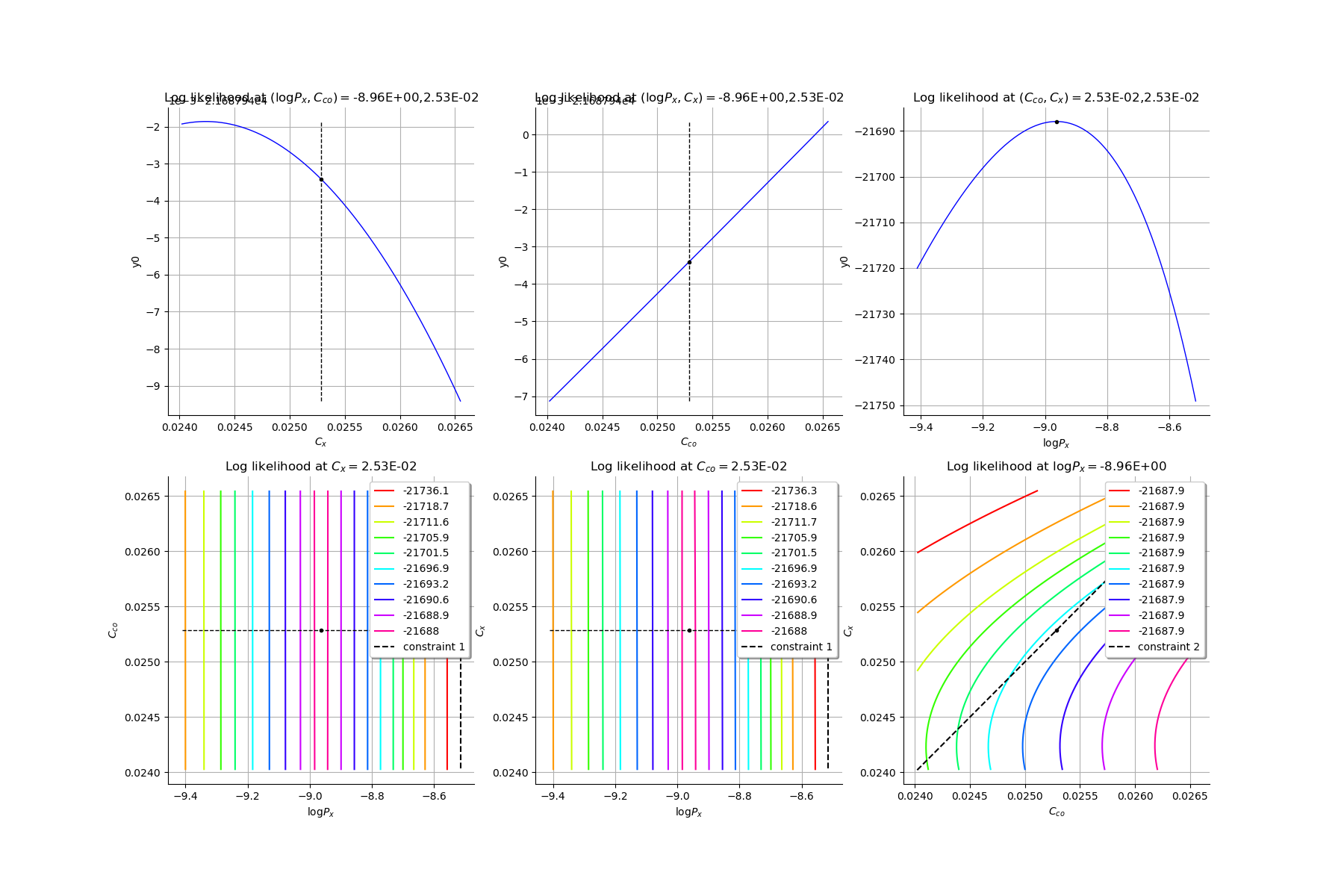
We use the Mankamo assumption. We use the maximum likelihood estimators of the Mankamo parameter. We want to get all the graphs of the likelihood function at the optimal Mankamo parameter.
We start by verifying that our starting point  for the optimization algorithm verifies the constraints!
[4]:
startingPoint = [5.0e-3, 0.51, 0.85]
print(myECLM.verifyMankamoConstraints(startingPoint))
False
If the point is not valid, we can ask for a valid one by giving  .
.
[5]:
startingPoint = myECLM.computeValidMankamoStartingPoint(0.7)
startingPoint
[5]:
[0.00018494,0.35,0.7]
Anyway, if the starting point is not valid, the function estimateMaxLikelihoodFromMankamo will automatically change it by itself.
[6]:
visuLikelihood = True
mankamoParam, generalParam, finalLogLikValue, graphesCol = myECLM.estimateMaxLikelihoodFromMankamo(startingPoint, visuLikelihood, verbose=False)
print('Mankamo parameter : ', mankamoParam)
print('general parameter : ', generalParam)
print('finalLogLikValue : ', finalLogLikValue)
Production of graphs
graph (Cco, Cx) = (Cco_optim, Cx_optim)
graph (logPx, Cx) = (logPx_optim, Cx_optim)
graph (logPx, Cco) = (logPx_optim, Cco_optim)
graph Cx = Cx_optim
graph Cco = Cco_optim
graph logPx = logPx_optim
Mankamo parameter :  [0.00036988020585009376, 0.00012801168928232786, 0.025285764581599247, 0.02528576558159925]
general parameter :  [0.9992086008496488, 0.04557096775442347, 0.045570968678919084, 0.2829364243530039, 0.7170635756469961]
finalLogLikValue :  -21687.94341532473
[8]:
gl = ot.GridLayout(2,3)
for i in range(6):
    gl.setGraph(i//3, i%3, graphesCol[i])
gl
[8]:
Compute the ECLM probabilities
[9]:
PEG_list = myECLM.computePEGall()
print('PEG_list = ', PEG_list)
print('')

PSG_list = myECLM.computePSGall()
print('PSG_list = ', PSG_list)
print('')

PES_list = myECLM.computePESall()
print('PES_list = ', PES_list)
print('')

PTS_list = myECLM.computePTSall()
print('PTS_list = ', PTS_list)
PEG_list =  [0.99775848489789, 0.00028415414547984774, 8.363578290642434e-06, 1.7370202481206713e-06, 3.9410426875976355e-07, 9.648993284764975e-08, 2.5440409734895204e-08, 7.210078132552946e-09]

PSG_list =  [0.9999999999999789, 0.00036988020585009104, 2.2089033674126945e-05, 4.001348637317756e-06, 7.671053746399512e-07, 1.5458083044999307e-07, 3.265048786744815e-08, 7.210078132552946e-09]

PES_list =  [0.99775848489789, 0.001989079018358934, 0.00017563514410349112, 6.07957086842235e-05, 1.3793649406591724e-05, 2.0262885898006447e-06, 1.7808286814426643e-07, 7.210078132552946e-09]

PTS_list =  [0.9999999999999792, 0.002241515102089318, 0.00025243608373038377, 7.680093962689269e-05, 1.6005230942669187e-05, 2.211581536077464e-06, 1.8529294627681937e-07, 7.210078132552946e-09]
Generate a sample of the parameters by Bootstrap
We use the bootstrap sampling to get a sample of total impact vectors. Each total impact vector value is associated to an optimal Mankamo parameter and an optimal general parameter. We fix the size of the bootstrap sample. We also fix the number of realisations after which the sample is saved. Each optimisation problem is initalised with the optimal parameter found for the total impact vector.
The sample is generated and saved in a csv file.
[10]:
Nbootstrap = 100
blockSize = 256
[11]:
startingPoint = mankamoParam[1:4]
fileNameSampleParam = 'sampleParamFromMankamo_{}.csv'.format(Nbootstrap)
myECLM.estimateBootstrapParamSampleFromMankamo(Nbootstrap, startingPoint, blockSize, fileNameSampleParam)
Create the sample of all the ECLM probabilities associated to the sample of the parameters.
[12]:
fileNameECLMProbabilities = 'sampleECLMProbabilitiesFromMankamo_{}.csv'.format(Nbootstrap)
myECLM.computeECLMProbabilitiesFromMankano(blockSize, fileNameSampleParam, fileNameECLMProbabilities)
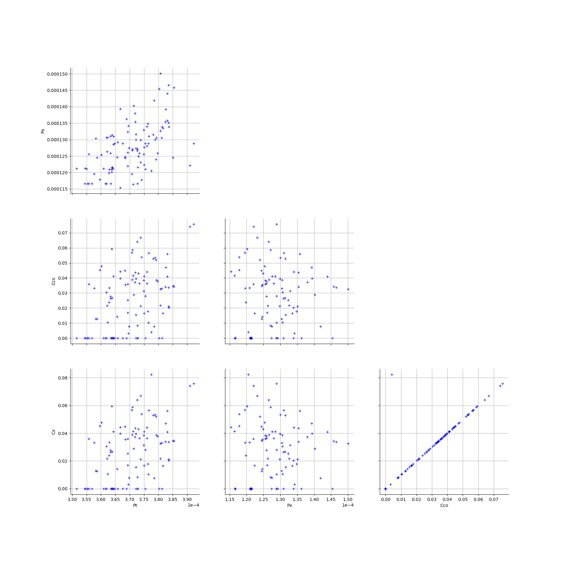
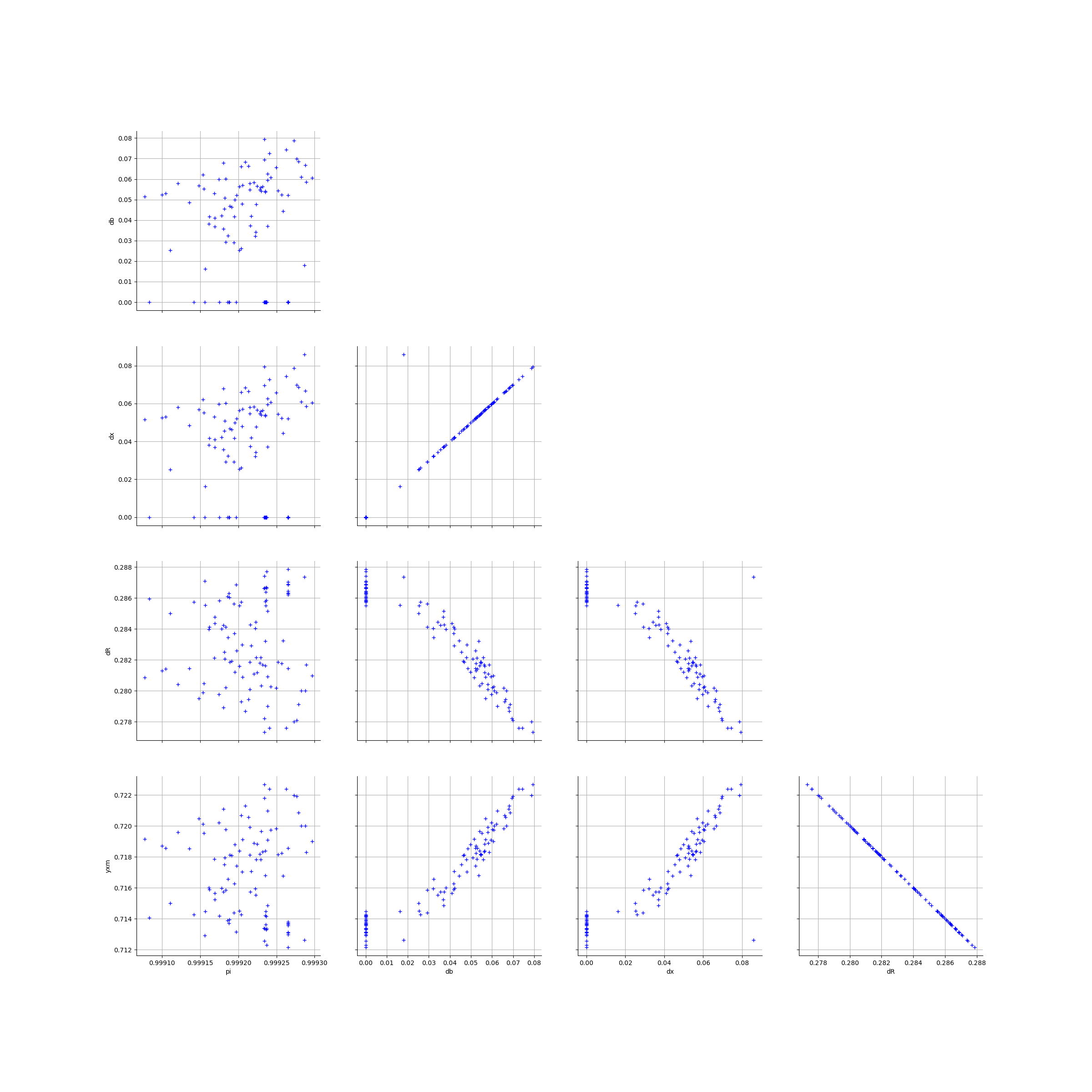
Graphically analyse the bootstrap sample of parameters
We create the Pairs graphs of the Mankamo and general parameters.
[13]:
graphPairsMankamoParam, graphPairsGeneralParam, graphMarg_list, descParam = myECLM.analyseGraphsECLMParam(fileNameSampleParam)
[14]:
graphPairsMankamoParam
[14]:
[15]:
graphPairsGeneralParam
[15]:
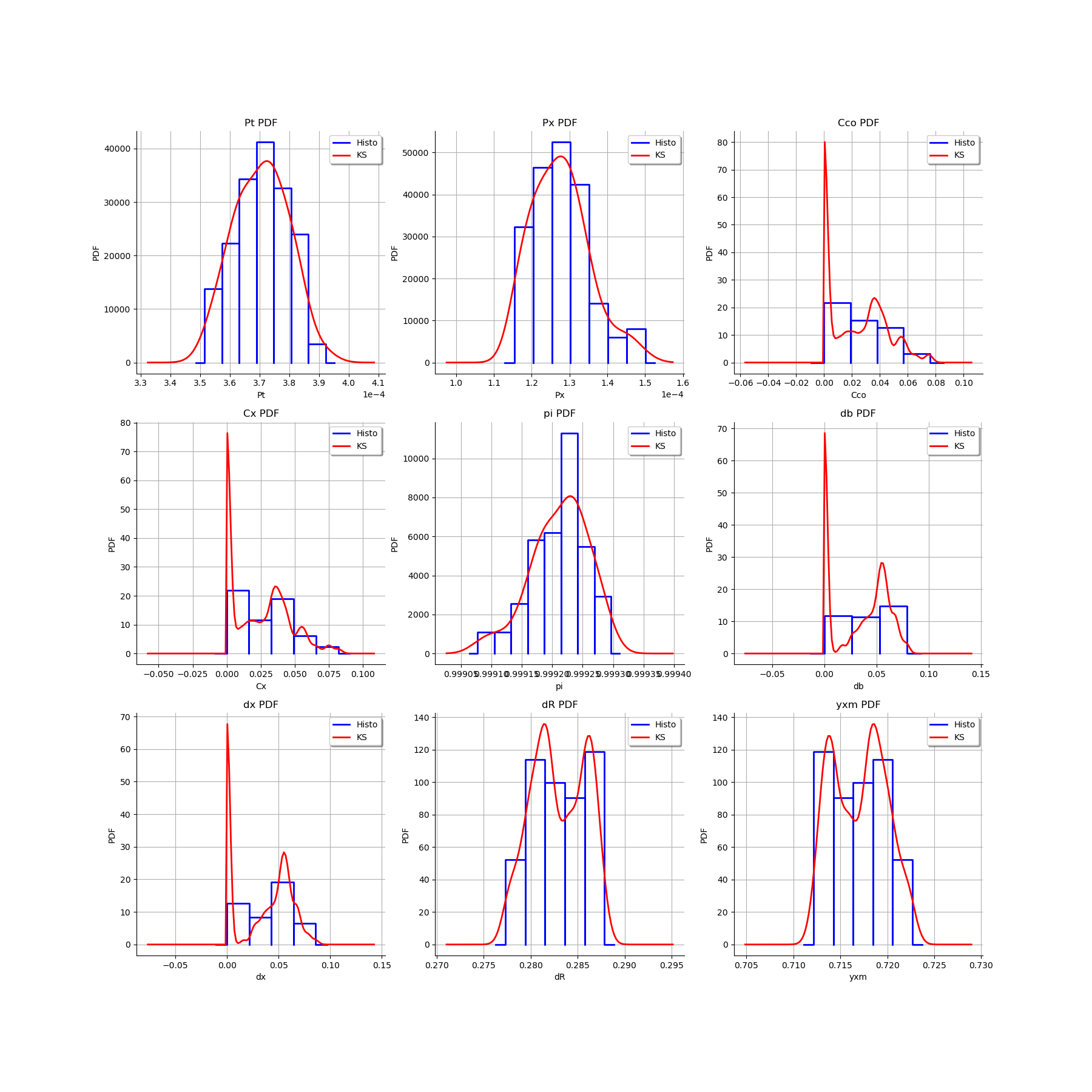
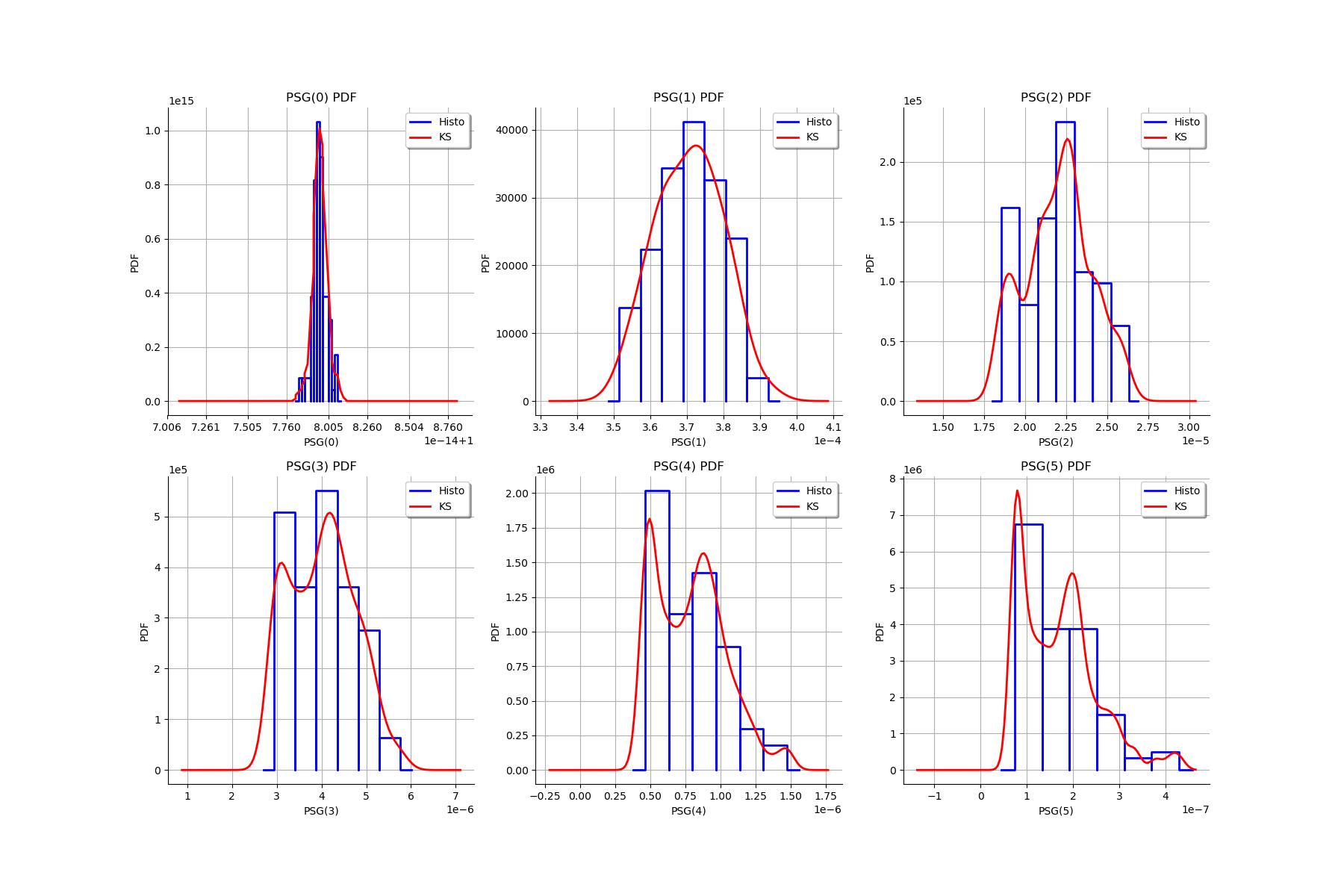
We estimate the distribution of each parameter with a Histogram and a normal kernel smoothing.
[16]:
gl = ot.GridLayout(3,3)
for k in range(len(graphMarg_list)):
    gl.setGraph(k//3, k%3, graphMarg_list[k])
gl
[16]:
Graphically analyse the bootstrap sample of the ECLM probabilities
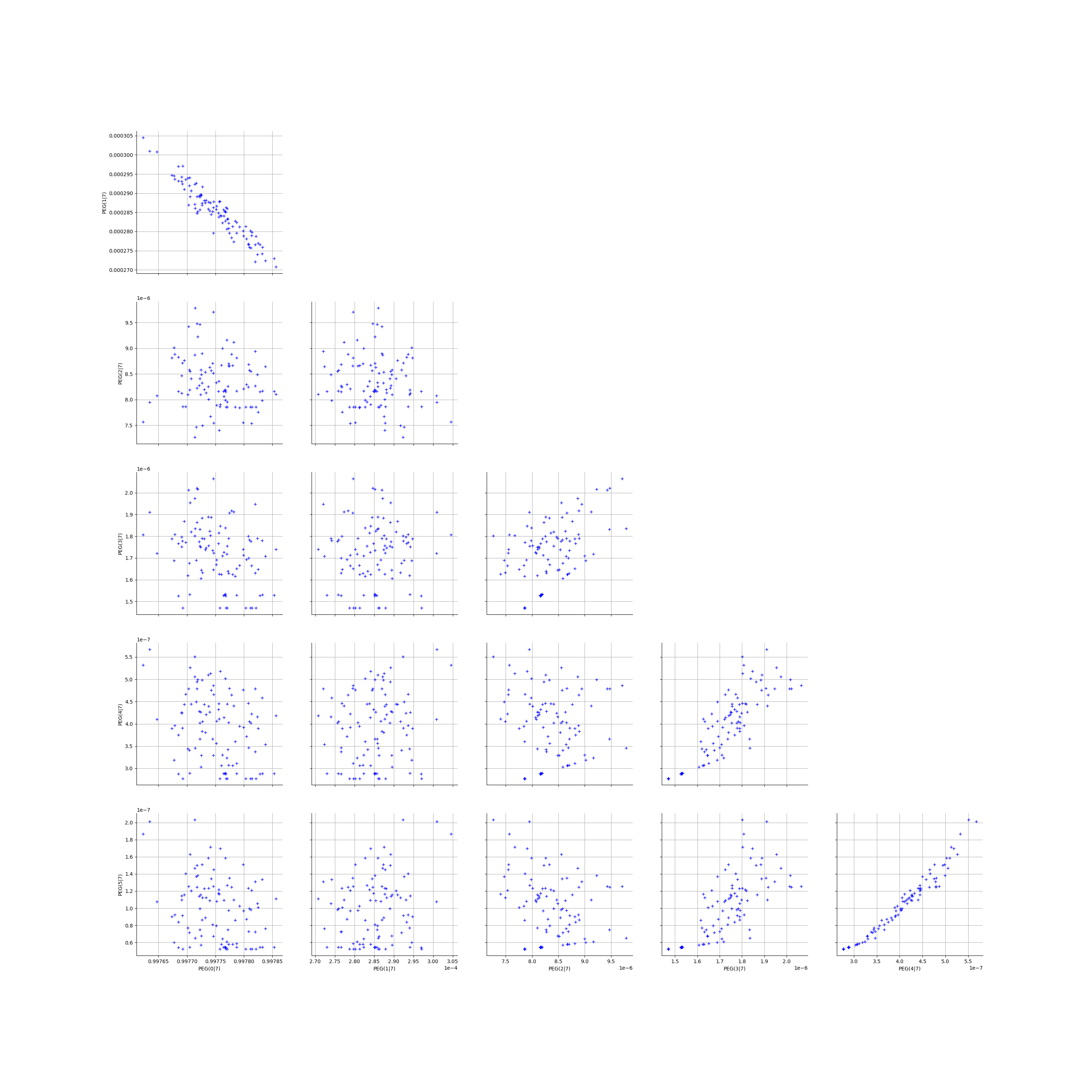
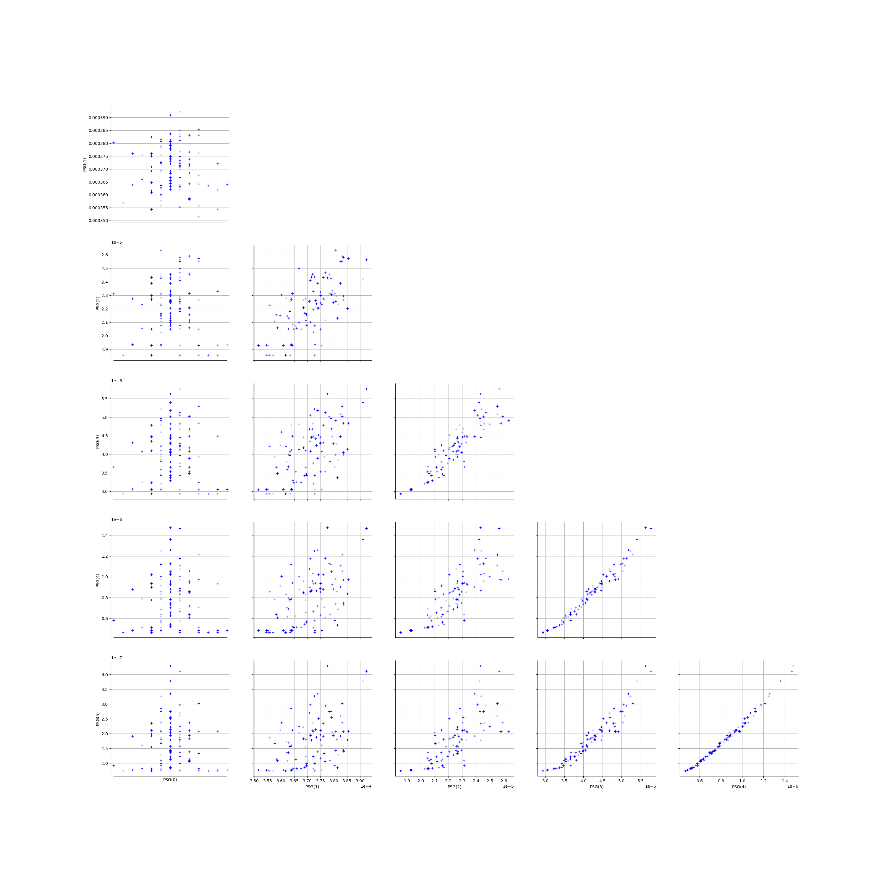
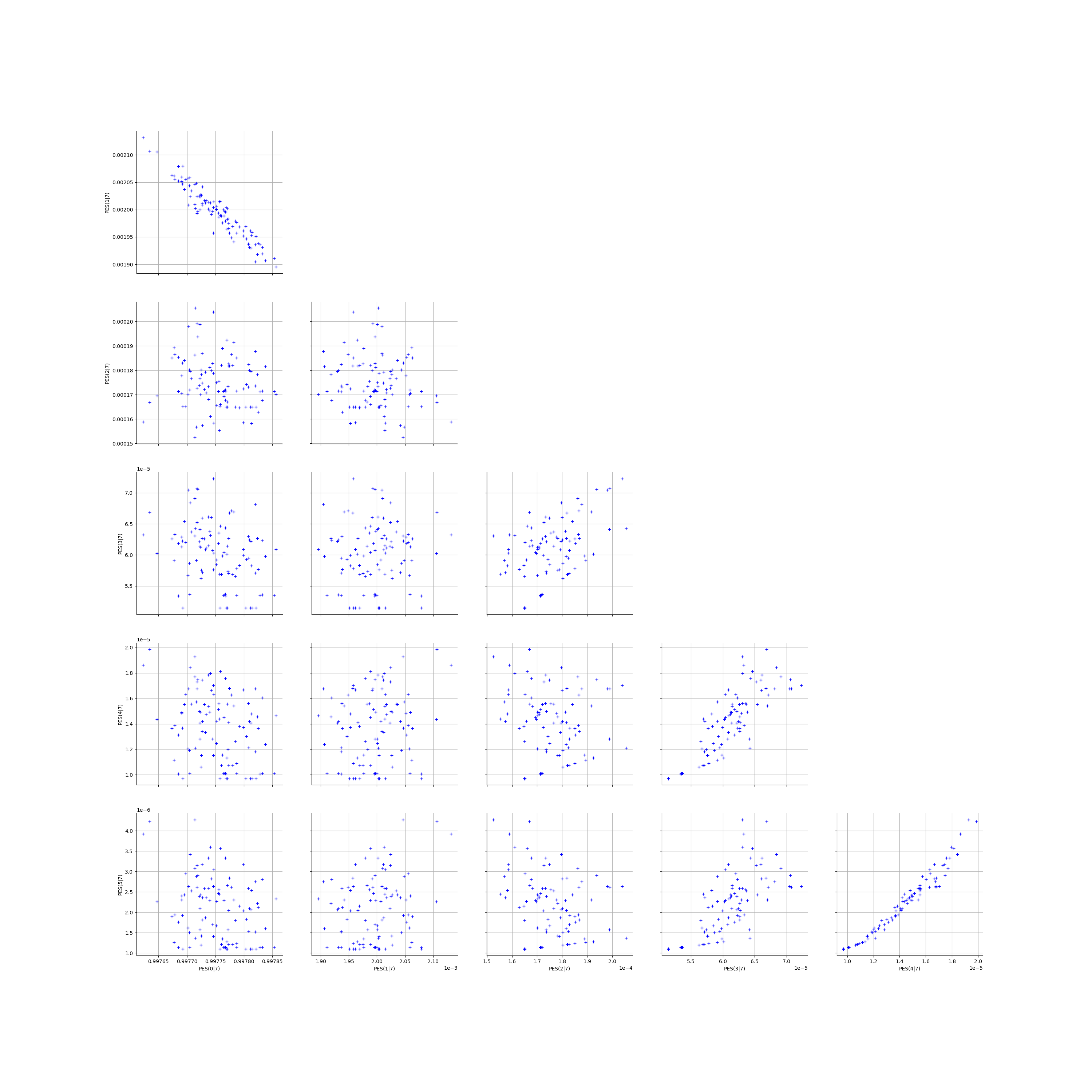
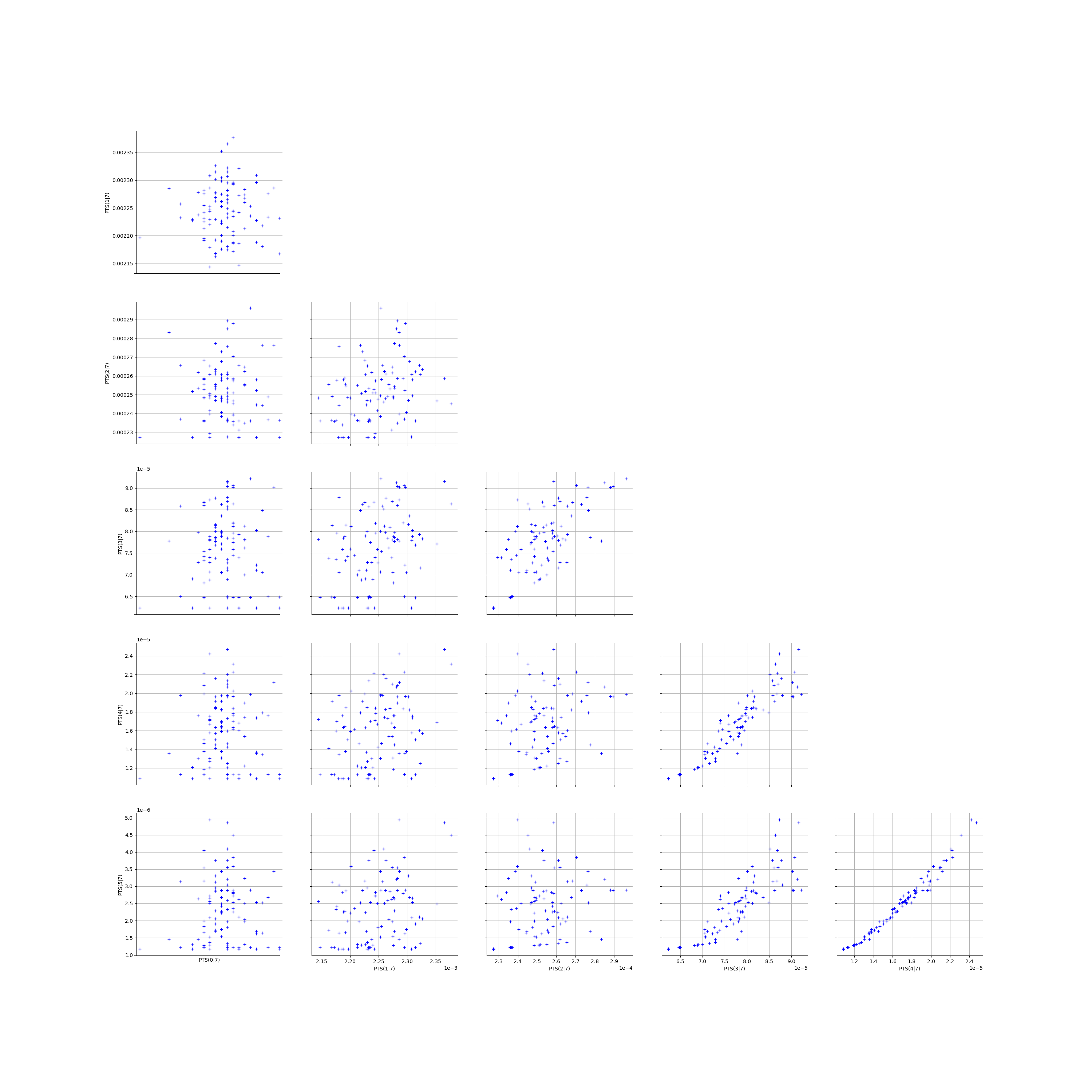
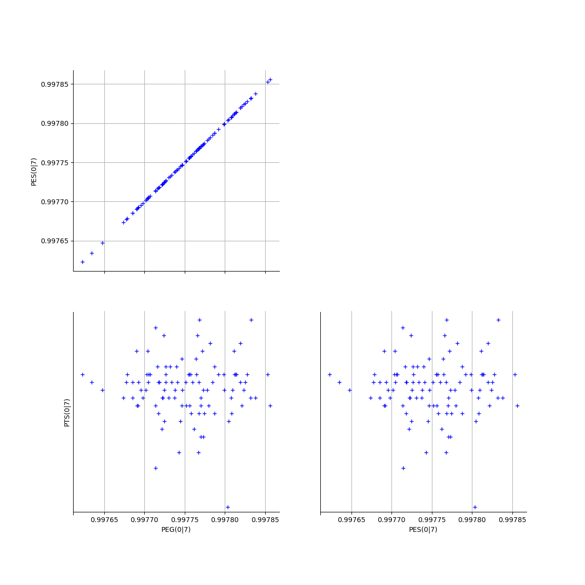
We create the Pairs graphs of all the ECLM probabilities. We limit the graphical study to the multiplicities lesser than  .
.
[17]:
kMax = 5

graphPairs_list, graphPEG_PES_PTS_list, graphMargPEG_list, graphMargPSG_list, graphMargPES_list, graphMargPTS_list, desc_list = myECLM.analyseGraphsECLMProbabilities(fileNameECLMProbabilities, kMax)
[18]:
descPairs = desc_list[0]
descPEG_PES_PTS = desc_list[1]
descMargPEG = desc_list[2]
descMargPSG = desc_list[3]
descMargPES = desc_list[4]
descMargPTS = desc_list[5]
[19]:
graphPairs_list[0]
[19]:
[20]:
graphPairs_list[1]
[20]:
[21]:
graphPairs_list[2]
[21]:
[22]:
graphPairs_list[3]
[22]:
[23]:
# Fix a k <=kMax
k = 0
graphPEG_PES_PTS_list[k]
[23]:
[24]:
len(graphMargPEG_list)
gl = ot.GridLayout(2,3)
for k in range(len(graphMargPEG_list)):
    gl.setGraph(k//3, k%3, graphMargPEG_list[k])
gl
[24]:

[25]:
gl = ot.GridLayout(2,3)
for k in range(len(graphMargPSG_list)):
    gl.setGraph(k//3, k%3, graphMargPSG_list[k])
gl
[25]:
[26]:
gl = ot.GridLayout(2,3)
for k in range(len(graphMargPES_list)):
    gl.setGraph(k//3, k%3, graphMargPES_list[k])
gl
[26]:
[27]:
gl = ot.GridLayout(2,3)
for k in range(len(graphMargPTS_list)):
    gl.setGraph(k//3, k%3, graphMargPTS_list[k])
gl
[27]:
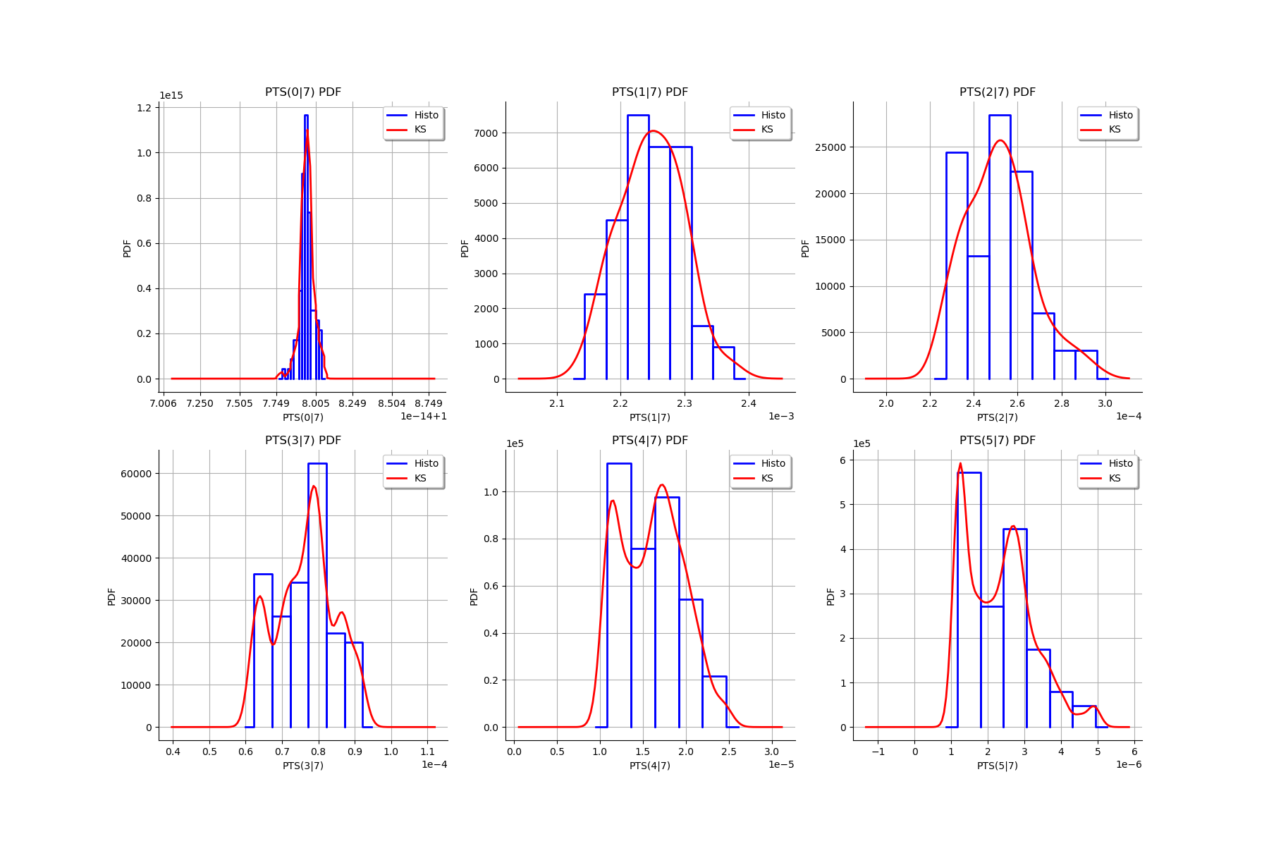
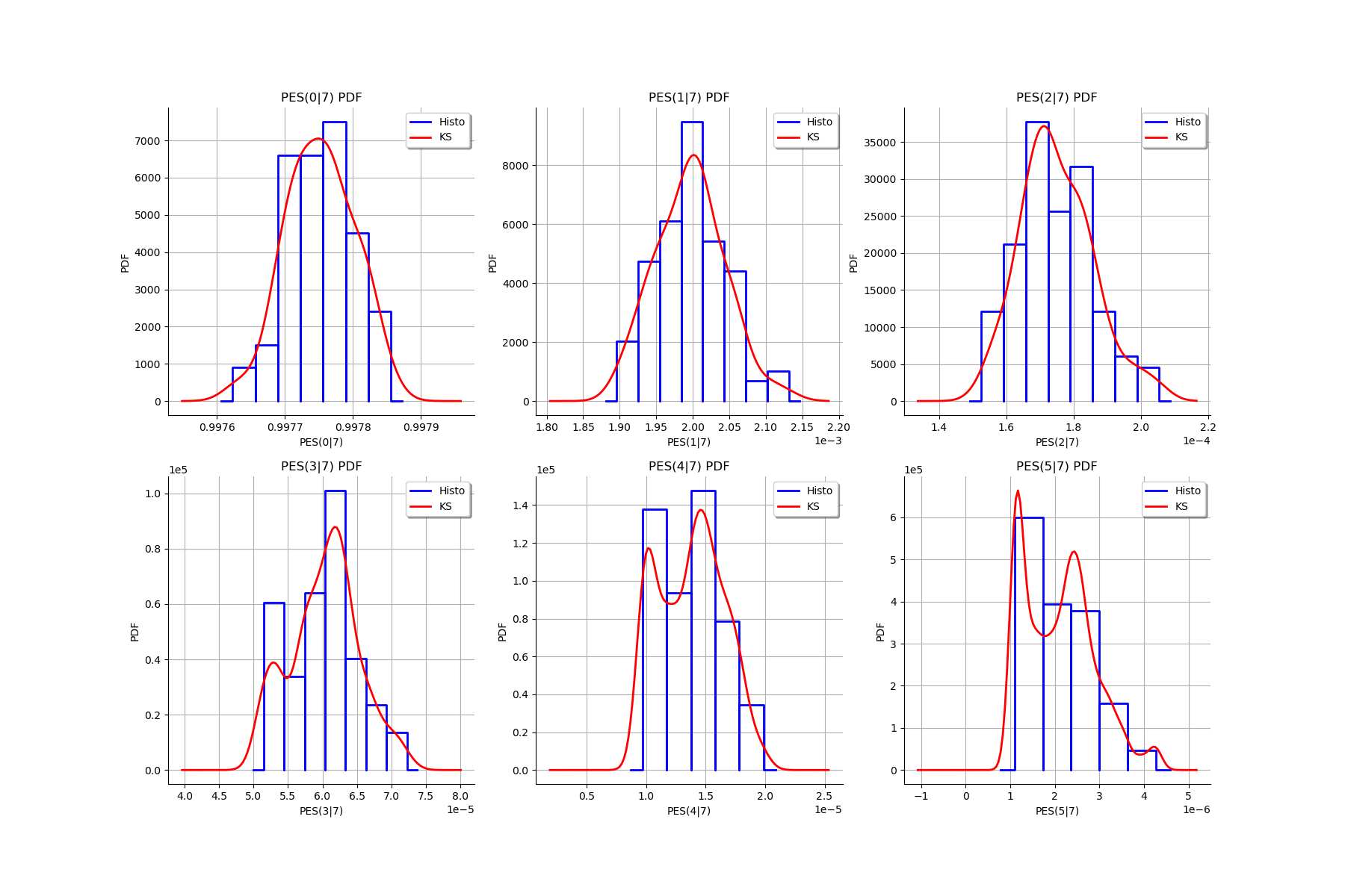
Fit a distribution to the ECLM probabilities
We fit a distribution among a given list to each ECLM probability. We test it with the Lilliefors test. We also compute the confidence interval of the specified level.
[28]:
factoryColl = [ot.BetaFactory(), ot.LogNormalFactory(), ot.GammaFactory()]
confidenceLevel = 0.9
IC_list, graphMarg_list, descMarg_list = myECLM.analyseDistECLMProbabilities(fileNameECLMProbabilities, kMax, confidenceLevel, factoryColl)

IC_PEG_list, IC_PSG_list, IC_PES_list, IC_PTS_list = IC_list
graphMargPEG_list, graphMargPSG_list, graphMargPES_list, graphMargPTS_list = graphMarg_list
descMargPEG, descMargPSG, descMargPES, descMargPTS = descMarg_list
Test de Lilliefors
==================
Ordre k= 0
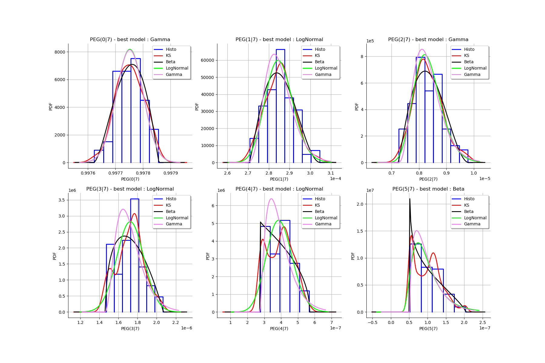
Best model PEG( 0 |n) : Gamma(k = 40897.7, lambda = 4.12706e+06, gamma = 0.987842) p-value = 0.6171742808798646
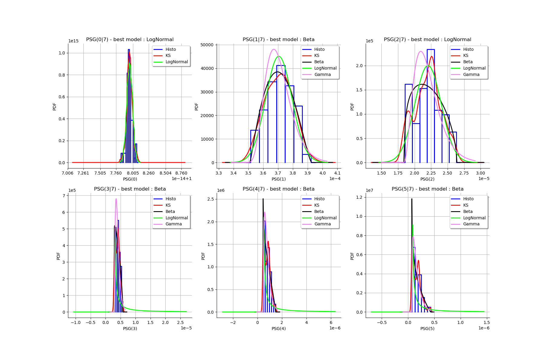
Best model PSG( 0 |n) : LogNormal(muLog = -26.0328, sigmaLog = 8.89975e-05, gamma = 1) p-value = 0.20976491862567812
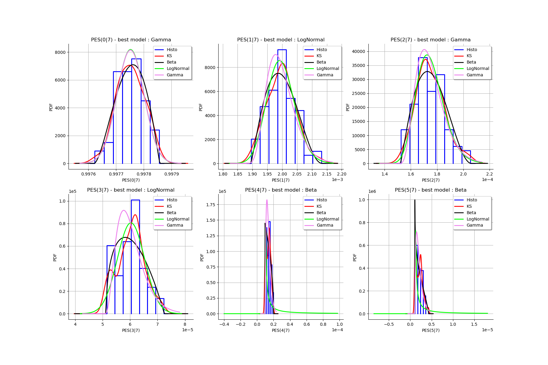
Best model PES( 0 |n) : Gamma(k = 40897.7, lambda = 4.12706e+06, gamma = 0.987842) p-value = 0.6026655560183257
Best model PTS( 0 |n) : LogNormal(muLog = -25.5223, sigmaLog = 5.38921e-05, gamma = 1) p-value = 0.055714285714285716
Test de Lilliefors
==================
Ordre k= 1
Best model PEG( 1 |n) : LogNormal(muLog = -9.34084, sigmaLog = 0.0760285, gamma = 0.00019719) p-value = 0.4729241877256318
Best model PSG( 1 |n) : Beta(alpha = 2.0922, beta = 2.36032, a = 0.000351093, b = 0.000392658) p-value = 0.6588921282798834
Best model PES( 1 |n) : LogNormal(muLog = -7.39493, sigmaLog = 0.0760285, gamma = 0.00138033) p-value = 0.47678142514011207
Best model PTS( 1 |n) : LogNormal(muLog = -6.71331, sigmaLog = 0.0401047, gamma = 0.00103231) p-value = 0.34352836879432624
Test de Lilliefors
==================
Ordre k= 2
Best model PEG( 2 |n) : Gamma(k = 5.00199, lambda = 4.37185e+06, gamma = 7.19275e-06) p-value = 0.5361736334405146
Best model PSG( 2 |n) : LogNormal(muLog = -3.89603, sigmaLog = 9.80732e-05, gamma = -0.0203003) p-value = 0.03296703296703297
Best model PES( 2 |n) : Gamma(k = 5.00199, lambda = 208183, gamma = 0.000151048) p-value = 0.5518354175070593
Best model PTS( 2 |n) : LogNormal(muLog = -9.63268, sigmaLog = 0.225222, gamma = 0.000184233) p-value = 0.07892107892107893
Test de Lilliefors
==================
Ordre k= 3
Best model PEG( 3 |n) : LogNormal(muLog = -9.1857, sigmaLog = 0.00137902, gamma = -0.000100772) p-value = 0.023976023976023976
Best model PSG( 3 |n) : Beta(alpha = 1.04361, beta = 1.66447, a = 2.90721e-06, b = 5.79377e-06) p-value = 0.000999000999000999
Best model PES( 3 |n) : LogNormal(muLog = -5.63481, sigmaLog = 0.00138518, gamma = -0.00351105) p-value = 0.022977022977022976
Best model PTS( 3 |n) : Beta(alpha = 1.12833, beta = 1.266, a = 6.20545e-05, b = 9.24656e-05) p-value = 0.00999000999000999
Test de Lilliefors
==================
Ordre k= 4
Best model PEG( 4 |n) : LogNormal(muLog = -13.6852, sigmaLog = 0.0678263, gamma = -7.48635e-07) p-value = 0.008991008991008992
Best model PSG( 4 |n) : Beta(alpha = 0.875666, beta = 1.8344, a = 4.55741e-07, b = 1.48579e-06) p-value = 0.005994005994005994
Best model PES( 4 |n) : Beta(alpha = 0.9944, beta = 1.48326, a = 9.60656e-06, b = 1.99598e-05) p-value = 0.000999000999000999
Best model PTS( 4 |n) : LogNormal(muLog = -13.3255, sigmaLog = 3.24704, gamma = 1.08751e-05) p-value = 0.07892107892107893
Test de Lilliefors
==================
Ordre k= 5
Best model PEG( 5 |n) : Beta(alpha = 0.829708, beta = 1.77852, a = 5.08153e-08, b = 2.04672e-07) p-value = 0.007992007992007992
Best model PSG( 5 |n) : Beta(alpha = 0.766877, beta = 2.10588, a = 7.03955e-08, b = 4.32479e-07) p-value = 0.06893106893106893
Best model PES( 5 |n) : Beta(alpha = 0.829708, beta = 1.77852, a = 1.06712e-06, b = 4.29812e-06) p-value = 0.003996003996003996
Best model PTS( 5 |n) : Beta(alpha = 0.818929, beta = 1.86304, a = 1.1321e-06, b = 4.97738e-06) p-value = 0.007992007992007992
[29]:
for k in range(len(IC_PEG_list)):
    print('IC_PEG_', k, ' = ', IC_PEG_list[k])

for k in range(len(IC_PSG_list)):
    print('IC_PSG_', k, ' = ', IC_PSG_list[k])

for k in range(len(IC_PES_list)):
    print('IC_PES_', k, ' = ', IC_PES_list[k])

for k in range(len(IC_PTS_list)):
    print('IC_PTS_', k, ' = ', IC_PTS_list[k])
IC_PEG_ 0  =  [0.997666, 0.997839]
IC_PEG_ 1  =  [0.000273448, 0.000297217]
IC_PEG_ 2  =  [7.49916e-06, 9.33129e-06]
IC_PEG_ 3  =  [1.47195e-06, 1.97351e-06]
IC_PEG_ 4  =  [2.69732e-07, 5.22866e-07]
IC_PEG_ 5  =  [4.86228e-08, 1.66726e-07]
IC_PSG_ 0  =  [1, 1]
IC_PSG_ 1  =  [0.000354533, 0.000386447]
IC_PSG_ 2  =  [1.85701e-05, 2.55343e-05]
IC_PSG_ 3  =  [2.86014e-06, 5.27513e-06]
IC_PSG_ 4  =  [4.39048e-07, 1.23337e-06]
IC_PSG_ 5  =  [6.54125e-08, 3.16607e-07]
IC_PES_ 0  =  [0.997666, 0.997839]
IC_PES_ 1  =  [0.00191414, 0.00208052]
IC_PES_ 2  =  [0.000157483, 0.000195957]
IC_PES_ 3  =  [5.15183e-05, 6.90728e-05]
IC_PES_ 4  =  [9.44105e-06, 1.83e-05]
IC_PES_ 5  =  [1.01772e-06, 3.5026e-06]
IC_PTS_ 0  =  [1, 1]
IC_PTS_ 1  =  [0.00216064, 0.00233412]
IC_PTS_ 2  =  [0.000226653, 0.00028162]
IC_PTS_ 3  =  [6.2362e-05, 9.01619e-05]
IC_PTS_ 4  =  [1.04958e-05, 2.22452e-05]
IC_PTS_ 5  =  [1.0748e-06, 3.96103e-06]
We draw all the estimated distributions and the title gives the best model.
[30]:
gl = ot.GridLayout(2,3)
for k in range(len(graphMargPEG_list)):
    gl.setGraph(k//3, k%3, graphMargPEG_list[k])
gl
[30]:
[31]:
gl = ot.GridLayout(2,3)
for k in range(len(graphMargPSG_list)):
    gl.setGraph(k//3, k%3, graphMargPSG_list[k])
gl
[31]:
[32]:
gl = ot.GridLayout(2,3)
for k in range(len(graphMargPES_list)):
        gl.setGraph(k//3, k%3, graphMargPES_list[k])
gl
[32]:
[33]:
gl = ot.GridLayout(2,3)
for k in range(len(graphMargPTS_list)):
    gl.setGraph(k//3, k%3, graphMargPTS_list[k])
gl
[33]:

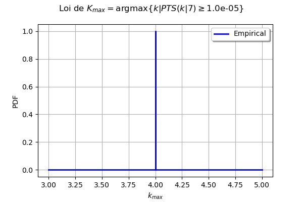
Analyse the minimal multiplicity which probability is greater than a given threshold
We fix p and we get the minimal multiplicity such that :

[34]:
p = 1.0e-5
nameSeuil = '10M5'
[35]:
kMax = myECLM.computeKMaxPTS(p)
print('kMax = ', kMax)
kMax = 4
Then we use the bootstrap sample of the Mankamo parameters to generate a sample of . We analyse the distribution of : we estimate it with the empirical distribution and we derive a confidence interval of order  .
.
[36]:
fileNameSampleParam = 'sampleParamFromMankamo_{}.csv'.format(Nbootstrap)
fileNameSampleKmax = 'sampleKmaxFromMankamo_{}_{}.csv'.format(Nbootstrap, nameSeuil)
gKmax = myECLM.computeAnalyseKMaxSample(p, blockSize, fileNameSampleParam, fileNameSampleKmax)
Intervalle de confiance de niveau 90%: [ 4.0 , 4.0 ]
[37]:
gKmax
[37]:
[ ]: