Extended Common Load Modelling

Import the required modules

import openturns as ot
from openturns.viewer import View
import oteclm

Description

We consider a common cause failure (CCF) groupe with n=7 identical and independent components. The total impact vector of this CCF group is estimated after N=1002100 demands or tests on the group.

n = 7
vectImpactTotal = ot.Indices(n+1)
vectImpactTotal[0] = 1000000
vectImpactTotal[1] = 2000
vectImpactTotal[2] = 200
vectImpactTotal[3] = 30
vectImpactTotal[4] = 20
vectImpactTotal[5] = 5
vectImpactTotal[6] = 0
vectImpactTotal[7] = 0

Create the ECLM class. We will use the Gauss Legendre quadrature algorithm to compute all the integrals of the ECLM model. The use of 50 points is sufficicient to reach a good precision.

myECLM = oteclm.ECLM(vectImpactTotal, ot.GaussLegendre([50]))

Estimate the optimal parameter

We use the Mankamo assumption. We use the maximum likelihood estimators of the Mankamo parameter. We want to get all the graphs of the likelihood function at the optimal Mankamo parameter.

We start by verifying that our starting point for the optimization algorithm verifies the constraints!

startingPoint = [5.0e-3, 0.51, 0.85]
print('Proposed starting point valid?: ', myECLM.verifyMankamoConstraints(startingPoint))

Proposed starting point valid?:  False

If the point is not valid, we can ask for a valid one by giving $C_x$.

startingPoint = myECLM.computeValidMankamoStartingPoint(0.7)
startingPoint

[0.00018494,0.35,0.7]

Anyway, if the starting point is not valid, the function estimateMaxLikelihoodFromMankamo will automatically change it by itself.

visuLikelihood = True
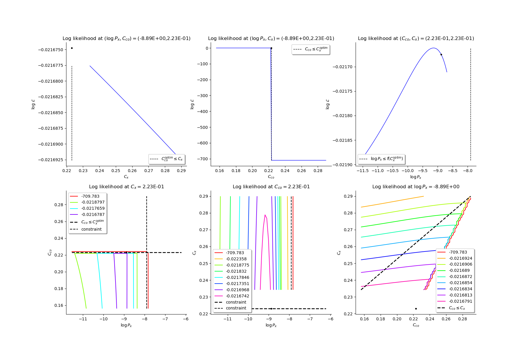
mankamoParam, generalParam, finalLogLikValue, graphesCol = myECLM.estimateMaxLikelihoodFromMankamo(startingPoint, visuLikelihood)
print('Mankamo parameter : ', mankamoParam)
print('general parameter : ', generalParam)
print('finalLogLikValue : ', finalLogLikValue)

Production of graphs
graph (Cco, Cx) = (Cco_optim, Cx_optim)
graph (logPx, Cx) = (logPx_optim, Cx_optim)
graph (logPx, Cco) = (logPx_optim, Cco_optim)
graph Cx = Cx_optim
graph Cco = Cco_optim
graph logPx = logPx_optim
Mankamo parameter :  [0.00036988020585009376, 0.00013842210875154897, 0.22303390975238369, 0.22303393403772004]
general parameter :  [0.9992677447205695, 0.1348884484265988, 0.13488845787842924, 0.25176209443183356, 0.7482379055681665]
finalLogLikValue :  -0.021674757309715593

Function to deactivate grid in GridLayout to make matplotlib happy

def deactivateGrid(gl):
    for i in range(gl.getNbRows()):
        for j in range(gl.getNbColumns()):
            g = gl.getGraph(i, j)
            g.setGrid(False)
            gl.setGraph(i, j, g)
    return gl

gl = ot.GridLayout(2, 3)
for i in range(6):
    g = graphesCol[i]
    gl.setGraph(i//3, i%3, g)

# Deactivate grid to make matplotlib happy
gl = deactivateGrid(gl)
view = View(gl)
view.show()

/usr/share/miniconda3/envs/test/lib/python3.11/site-packages/openturns/viewer.py:526: UserWarning: No contour levels were found within the data range.
  contourset = self._ax[0].contour(X, Y, Z, **contour_kw)

Compute the ECLM probabilities

PEG_list = myECLM.computePEGall()
print('PEG_list = ', PEG_list)
print('')

PSG_list = myECLM.computePSGall()
print('PSG_list = ', PSG_list)
print('')

PES_list = myECLM.computePESall()
print('PES_list = ', PES_list)
print('')

PTS_list = myECLM.computePTSall()
print('PTS_list = ', PTS_list)

PEG_list =  [0.9979125079558581, 0.0002576153710104107, 7.195205323914234e-06, 2.1683719809534964e-06, 1.0445342267102284e-06, 7.12809140752598e-07, 6.792244923025189e-07, 9.098545767821039e-07]

PSG_list =  [1.0, 0.00036988020585009094, 3.991647594160468e-05, 1.4250116278302177e-05, 6.130489702657682e-06, 2.9811127021397395e-06, 1.5890790690846228e-06, 9.098545767821039e-07]

PES_list =  [0.9979125079558581, 0.001803307597072875, 0.0001510993118021989, 7.589301933337237e-05, 3.6558697934858e-05, 1.4968991955804558e-05, 4.754571446117632e-06, 9.098545767821039e-07]

PTS_list =  [1.0, 0.002087492044122008, 0.0002841844470491336, 0.00013308513524693465, 5.719211591356229e-05, 2.0633417978704295e-05, 5.6644260228997354e-06, 9.098545767821039e-07]

Generate a sample of the parameters by Bootstrap

We use the bootstrap sampling to get a sample of total impact vectors. Each total impact vector value is associated to an optimal Mankamo parameter and an optimal general parameter. We fix the size of the bootstrap sample. We also fix the number of realisations after which the sample is saved. Each optimisation problem is initalised with the optimal parameter found for the total impact vector.

The sample is generated and saved in a csv file.

Nbootstrap = 100

startingPoint = mankamoParam[1:4]
fileNameSampleParam = 'sampleParamFromMankamo_{}.csv'.format(Nbootstrap)
# We use the parallelisation
parallel = True
blocksize = 256
myECLM.estimateBootstrapParamSampleFromMankamo(Nbootstrap, startingPoint, fileNameSampleParam, blocksize, parallel)

# Create the sample of all the ECLM probabilities associated to the sample of the parameters.

fileNameECLMProbabilities = 'sampleECLMProbabilitiesFromMankamo_{}.csv'.format(Nbootstrap)
# We use the parallelisation
parallel = True
myECLM.computeECLMProbabilitiesFromMankano(fileNameSampleParam, fileNameECLMProbabilities, blocksize, parallel)

Graphically analyse the bootstrap sample of parameters

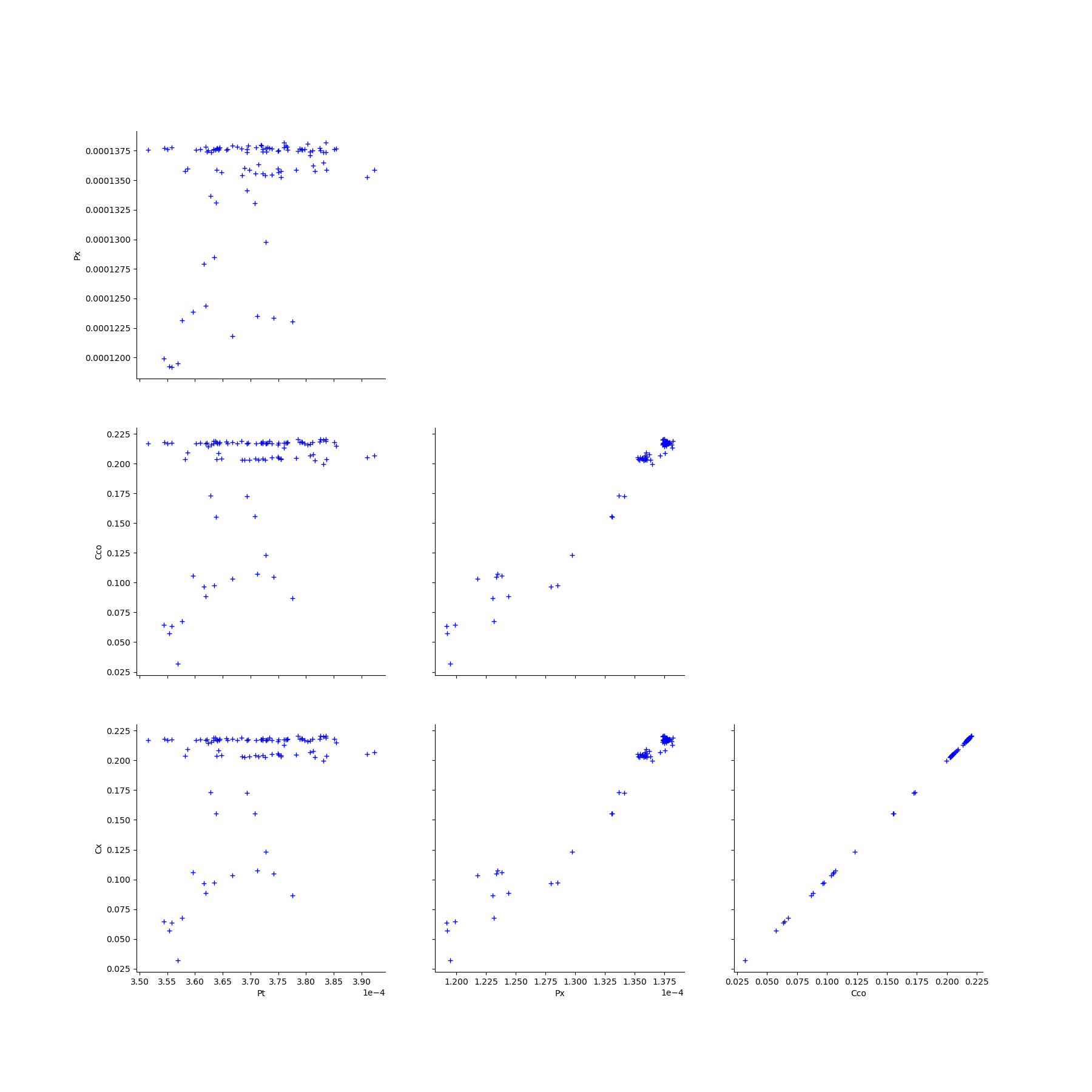
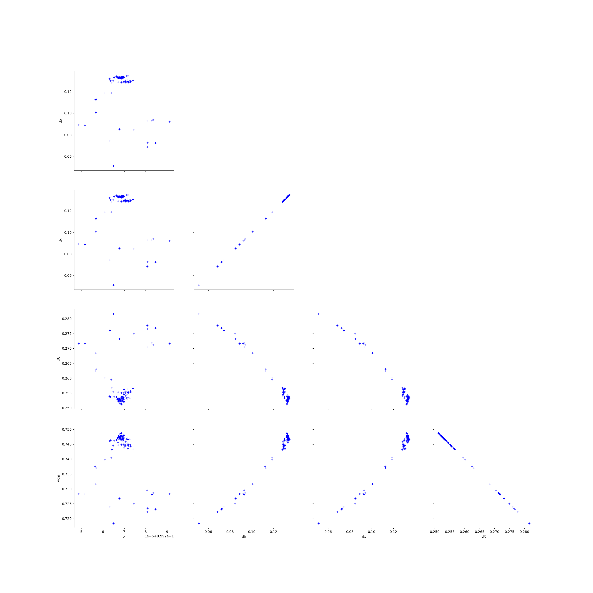
We create the Pairs graphs of the Mankamo and general parameters.

graphPairsMankamoParam, graphPairsGeneralParam, graphMarg_list, descParam = myECLM.analyseGraphsECLMParam(fileNameSampleParam)

Deactivate grid to make matplotlib happy

graphPairsMankamoParam = deactivateGrid(graphPairsMankamoParam)

view = View(graphPairsMankamoParam)
view.show()

Deactivate grid to make matplotlib happy

graphPairsGeneralParam = deactivateGrid(graphPairsGeneralParam)

view = View(graphPairsGeneralParam)
view.show()

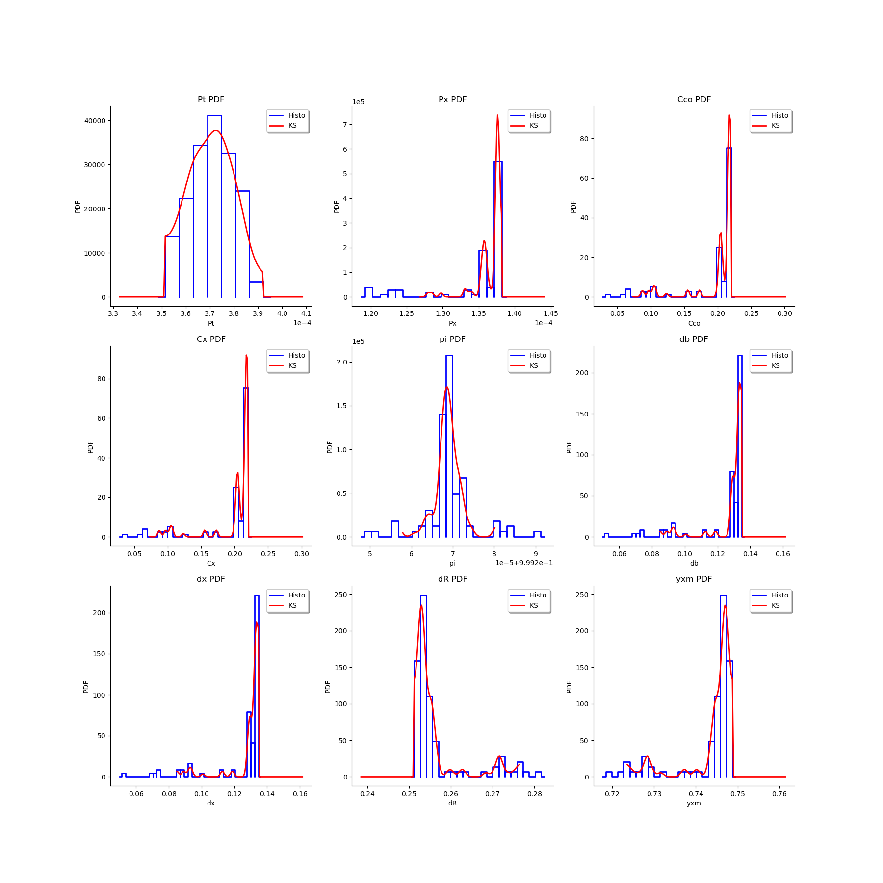
# We estimate the distribution of each parameter with a Histogram and a normal kernel smoothing.

gl = ot.GridLayout(3,3)
for k in range(len(graphMarg_list)):
    g = graphMarg_list[k]
    gl.setGraph(k//3, k%3, g)

# Deactivate grid to make matplotlib happy
gl = deactivateGrid(gl)
view = View(gl)
view.show()

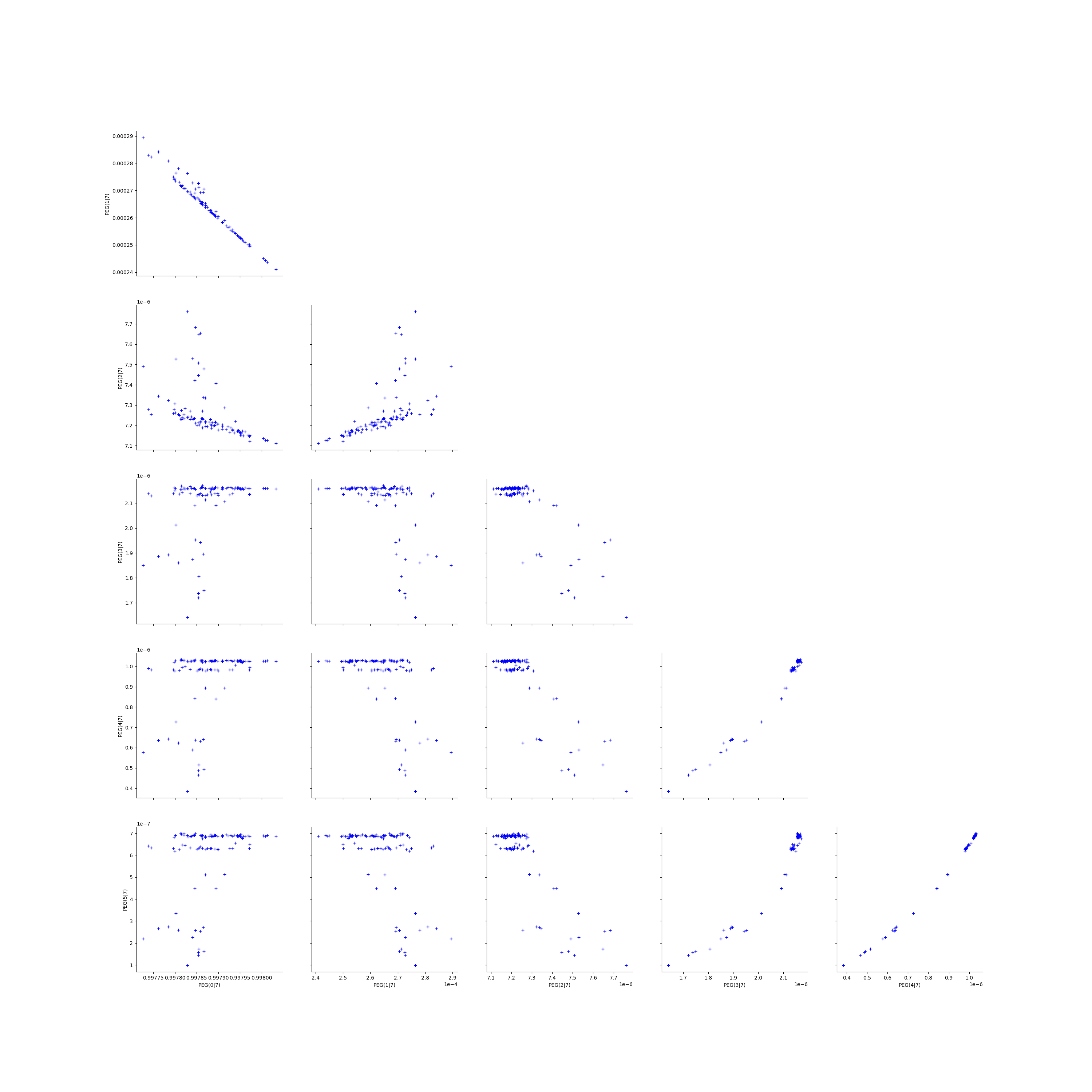
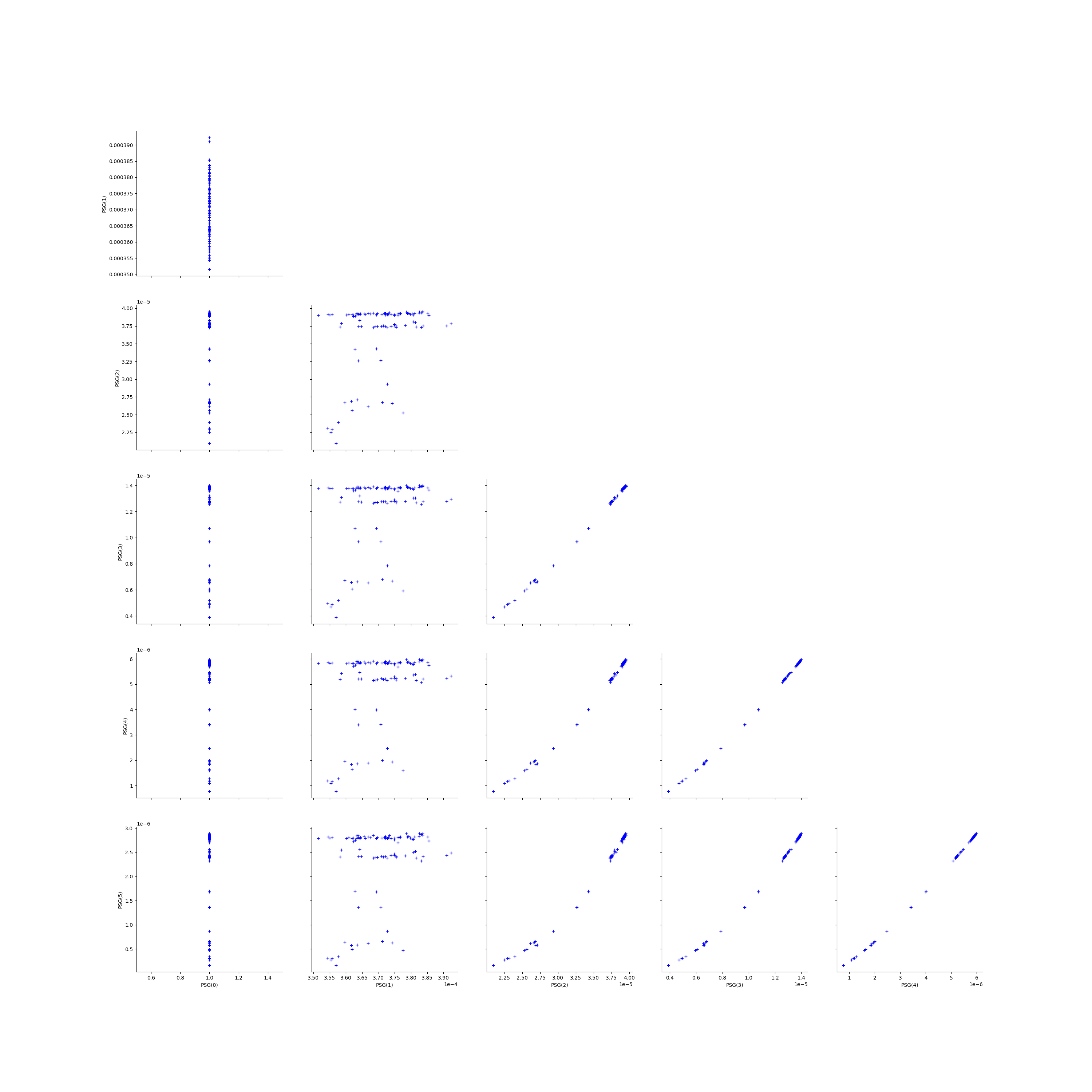
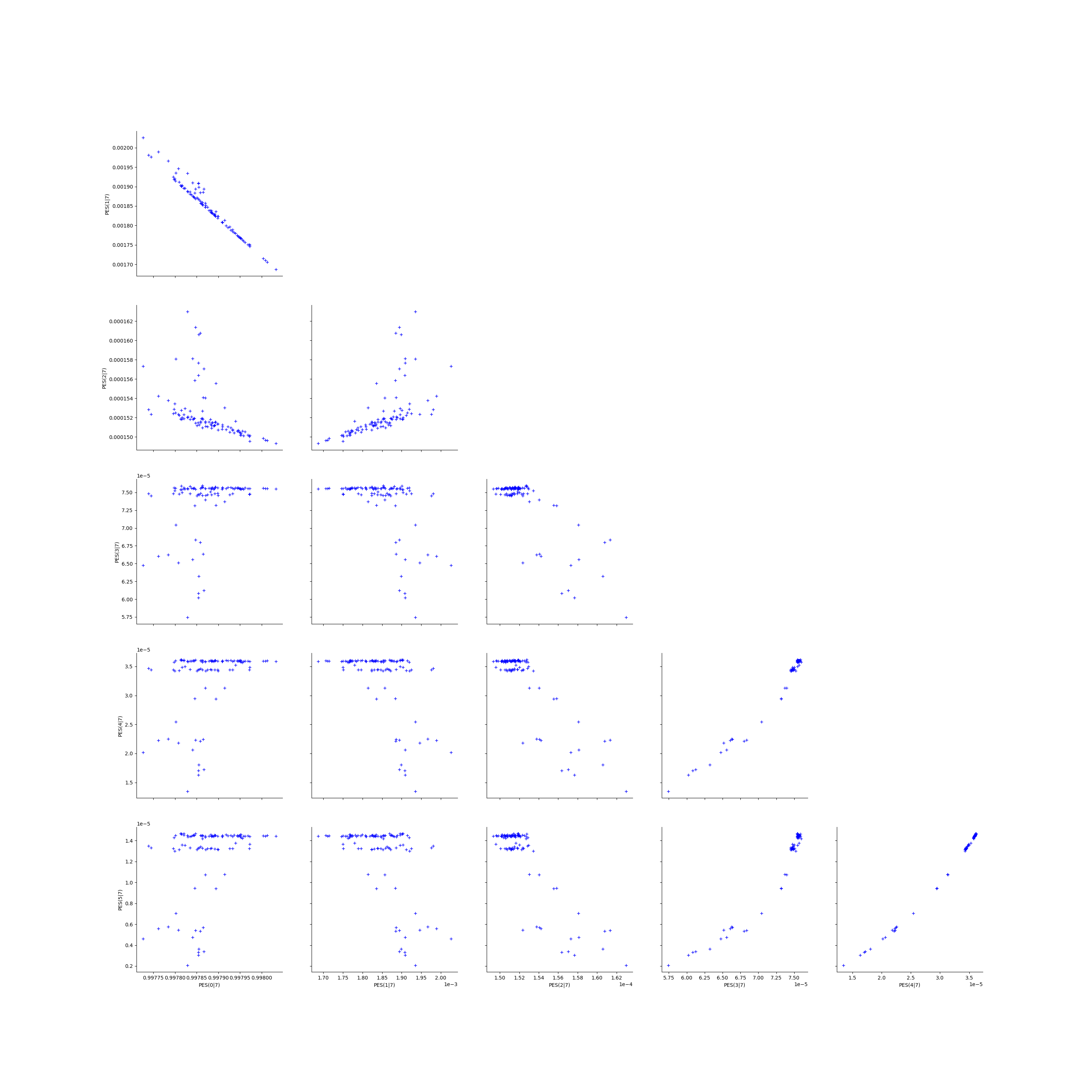
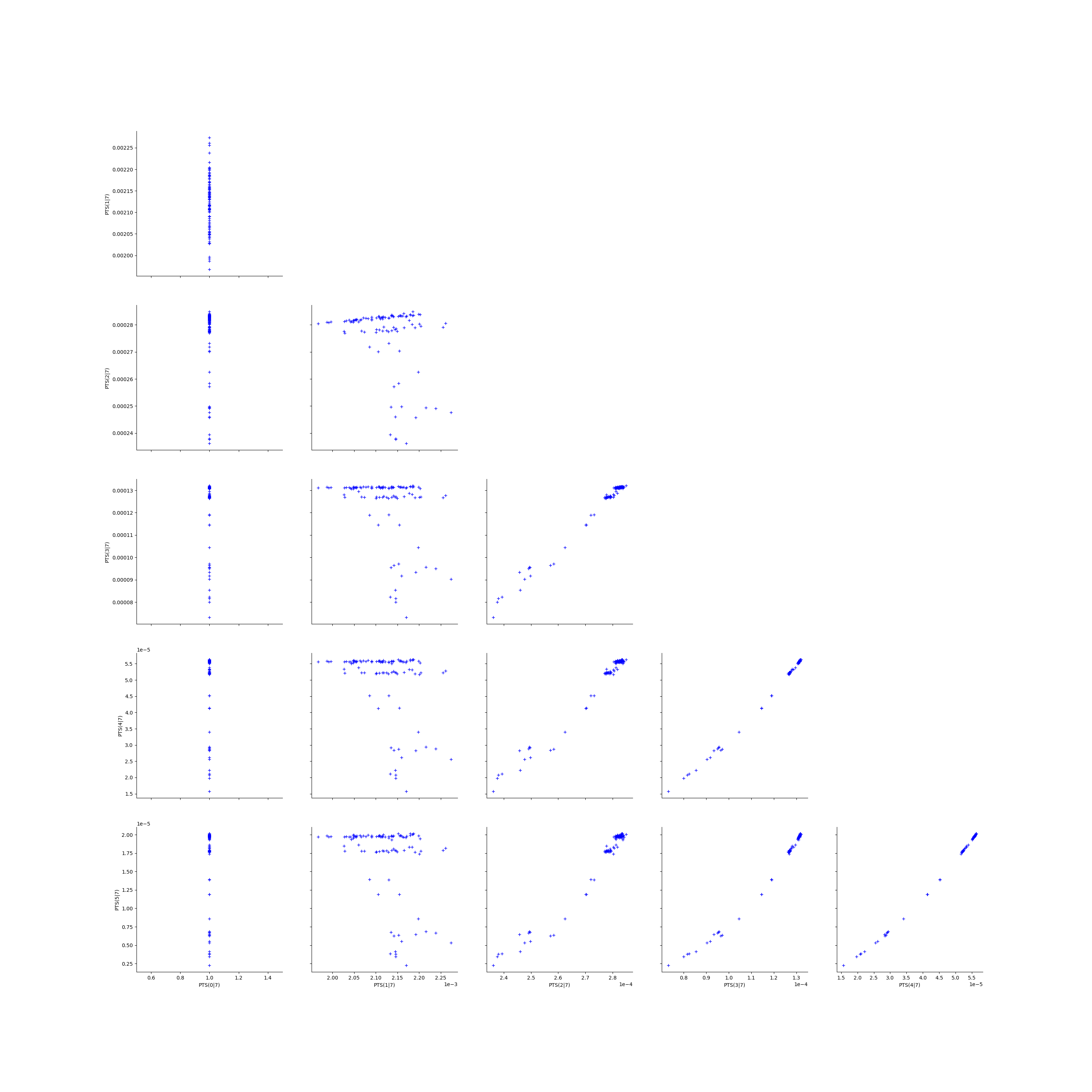
Graphically analyse the bootstrap sample of the ECLM probabilities

We create the Pairs graphs of all the ECLM probabilities. We limit the graphical study to the multiplicities lesser than .

kMax = 5

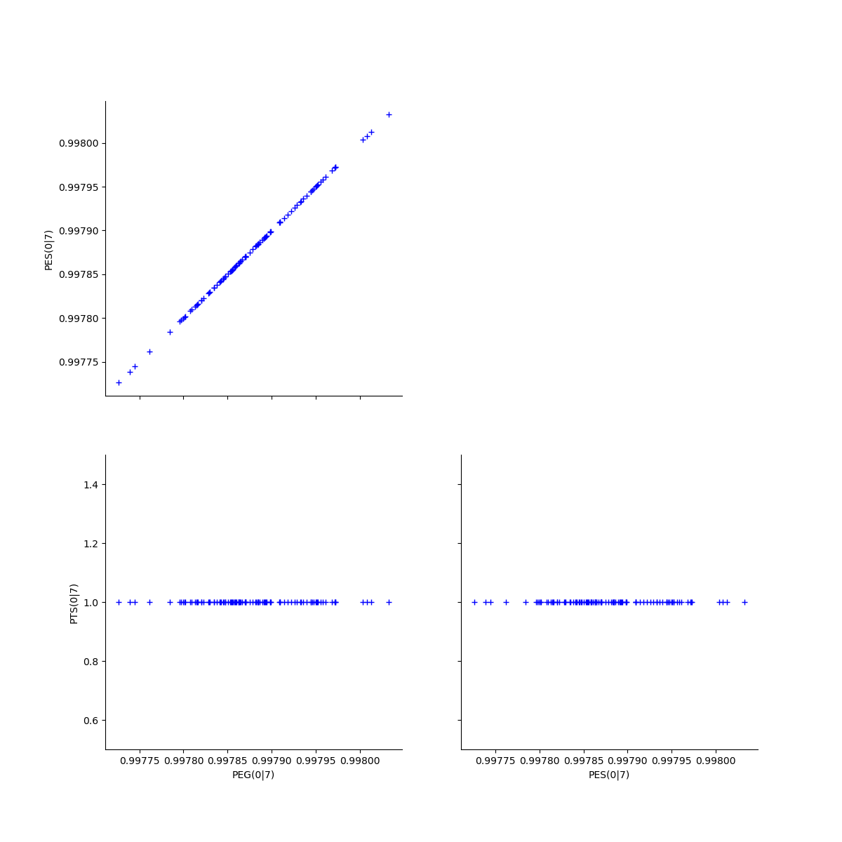
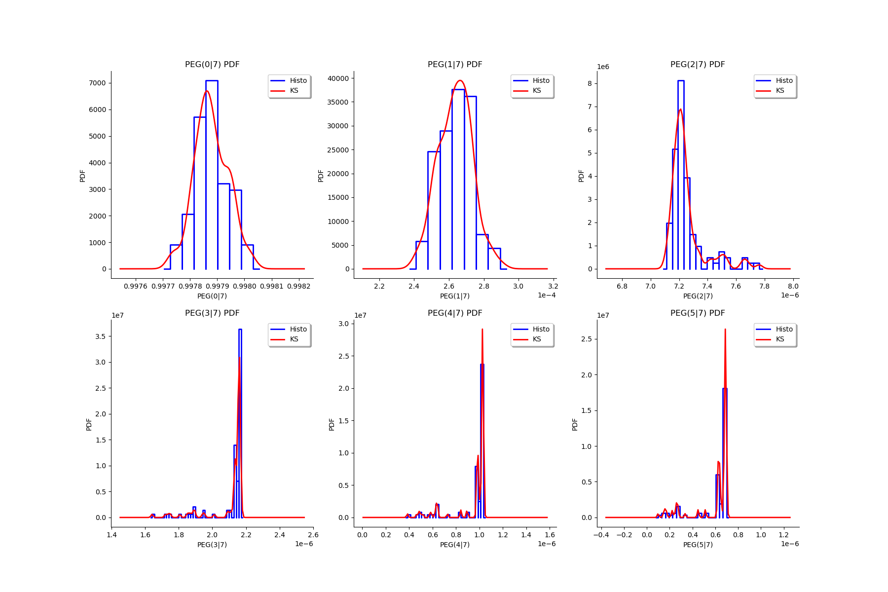
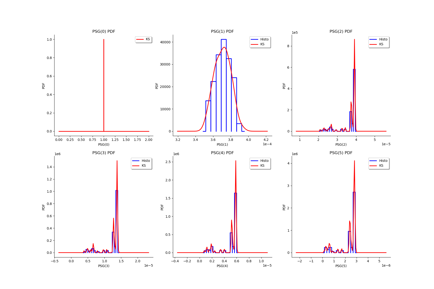
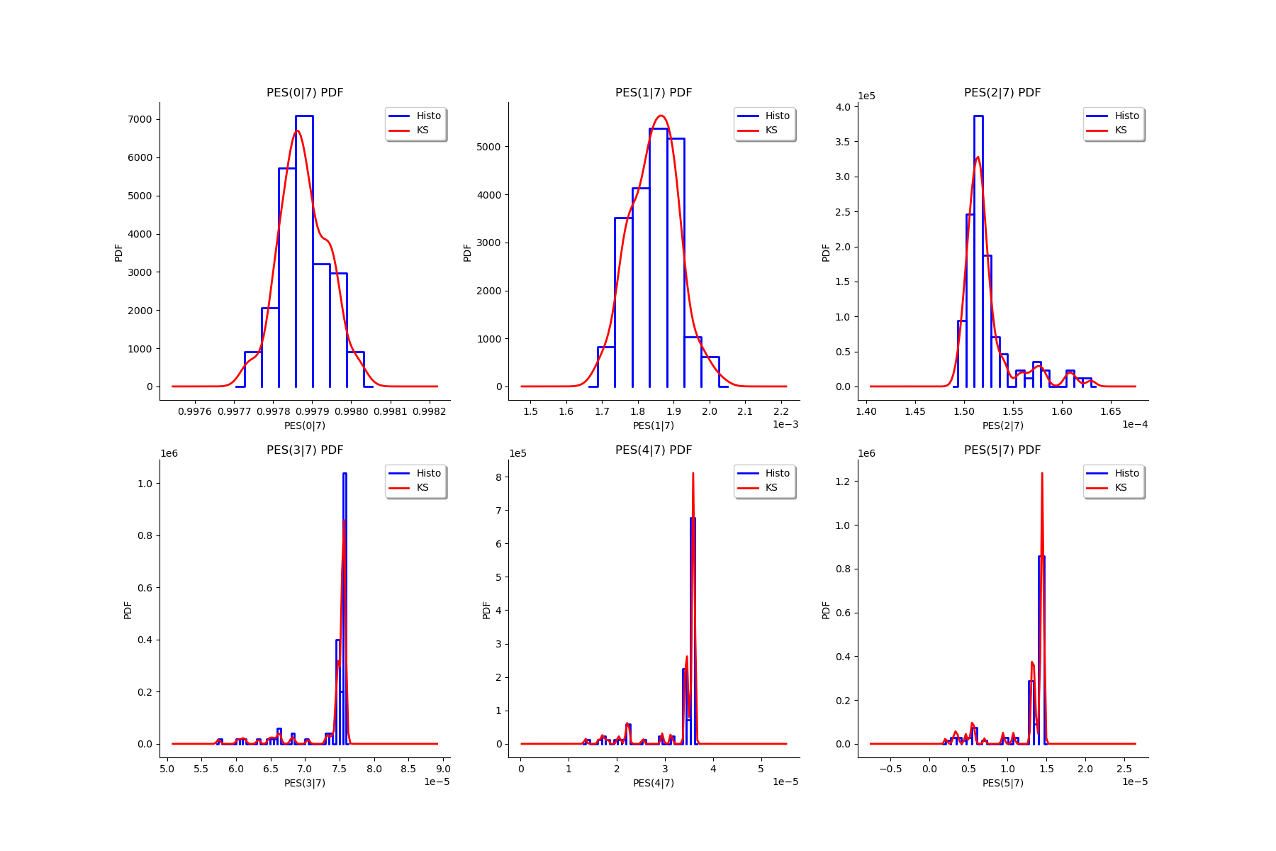
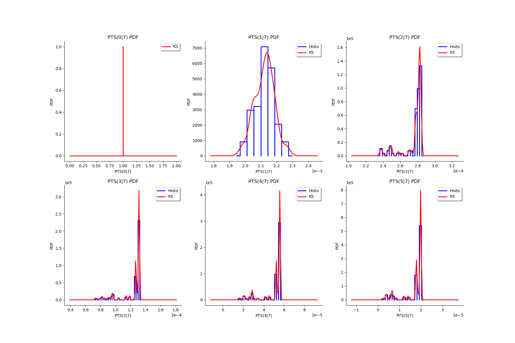
graphPairs_list, graphPEG_PES_PTS_list, graphMargPEG_list, graphMargPSG_list, graphMargPES_list, graphMargPTS_list, desc_list = myECLM.analyseGraphsECLMProbabilities(fileNameECLMProbabilities, kMax)

descPairs = desc_list[0]
descPEG_PES_PTS = desc_list[1]
descMargPEG = desc_list[2]
descMargPSG = desc_list[3]
descMargPES = desc_list[4]
descMargPTS = desc_list[5]

Deactivate grid to make matplotlib happy

graphPairs_list[0] = deactivateGrid(graphPairs_list[0])

view = View(graphPairs_list[0])
view.show()

Deactivate grid to make matplotlib happy

graphPairs_list[1] = deactivateGrid(graphPairs_list[1])

view = View(graphPairs_list[1])
view.show()

Deactivate grid to make matplotlib happy

graphPairs_list[2] = deactivateGrid(graphPairs_list[2])

view = View(graphPairs_list[2])
view.show()

Deactivate grid to make matplotlib happy

graphPairs_list[3] = deactivateGrid(graphPairs_list[3])

view = View(graphPairs_list[3])
view.show()

Fix a k <=kMax

k = 0
gl = graphPEG_PES_PTS_list[k]
gl = deactivateGrid(gl)
view = View(gl)
view.show()

len(graphMargPEG_list)
gl = ot.GridLayout(2, 3)
for k in range(6):
    g = graphMargPEG_list[k]
    gl.setGraph(k//3, k%3, g)

# Deactivate grid to make matplotlib happy
gl = deactivateGrid(gl)
view = View(gl)
view.show()

gl = ot.GridLayout(2, 3)
for k in range(6):
    g = graphMargPSG_list[k]
    gl.setGraph(k//3, k%3, g)

# Deactivate grid to make matplotlib happy
gl = deactivateGrid(gl)
view = View(gl)
view.show()

gl = ot.GridLayout(2, 3)
for k in range(6):
    g = graphMargPES_list[k]
    gl.setGraph(k//3, k%3, g)

# Deactivate grid to make matplotlib happy
gl = deactivateGrid(gl)
view = View(gl)
view.show()

gl = ot.GridLayout(2, 3)
for k in range(6):
    g = graphMargPTS_list[k]
    gl.setGraph(k//3, k%3, g)

# Deactivate grid to make matplotlib happy
gl = deactivateGrid(gl)
view = View(gl)
view.show()

Fit a distribution to the ECLM probabilities

We fit a distribution among a given list to each ECLM probability. We test it with the Lilliefors test. We also compute the confidence interval of the specified level.

factoryColl = [ot.BetaFactory(), ot.LogNormalFactory(), ot.GammaFactory()]
confidenceLevel = 0.9
IC_list, graphMarg_list, descMarg_list = myECLM.analyseDistECLMProbabilities(fileNameECLMProbabilities, kMax, confidenceLevel, factoryColl)

IC_PEG_list, IC_PSG_list, IC_PES_list, IC_PTS_list = IC_list
graphMargPEG_list, graphMargPSG_list, graphMargPES_list, graphMargPTS_list = graphMarg_list
descMargPEG, descMargPSG, descMargPES, descMargPTS = descMarg_list

Test de Lilliefors
==================

Ordre k= 0
PEG...
Best model PEG( 0 |n) :  LogNormal(muLog = -6.50028, sigmaLog = 0.0405954, gamma = 0.996374) p-value =  0.3558576569372251
PSG...
Not able to fit any model
PES...
Best model PES( 0 |n) :  LogNormal(muLog = -6.50028, sigmaLog = 0.0405954, gamma = 0.996374) p-value =  0.38692211578508956
PTS...
Not able to fit any model

Test de Lilliefors
==================

Ordre k= 1
PEG...
Best model PEG( 1 |n) :  LogNormal(muLog = -6.30661, sigmaLog = 0.00515303, gamma = -0.00156058) p-value =  0.6777289084366253
PSG...
Best model PSG( 1 |n) :  Beta(alpha = 2.0922, beta = 2.36032, a = 0.000351093, b = 0.000392658) p-value =  0.6527104451300132
PES...
Best model PES( 1 |n) :  LogNormal(muLog = -4.36066, sigmaLog = 0.00515283, gamma = -0.0109246) p-value =  0.6784673052894629
PTS...
Best model PTS( 1 |n) :  LogNormal(muLog = 1.45148, sigmaLog = 1.43078e-05, gamma = -4.26733) p-value =  0.21882217090069284

Test de Lilliefors
==================

Ordre k= 2
PEG...
Best model PEG( 2 |n) :  LogNormal(muLog = -15.859, sigmaLog = 0.63656, gamma = 7.09189e-06) p-value =  0.001998001998001998
PSG...
Best model PSG( 2 |n) :  Beta(alpha = 0.919147, beta = 0.179811, a = 2.07667e-05, b = 3.97147e-05) p-value =  0.20523809523809525
PES...
Best model PES( 2 |n) :  LogNormal(muLog = -12.8144, sigmaLog = 0.63656, gamma = 0.00014893) p-value =  0.000999000999000999
PTS...
Best model PTS( 2 |n) :  LogNormal(muLog = 0.940769, sigmaLog = 4.76938e-06, gamma = -2.56167) p-value =  0.001998001998001998

Test de Lilliefors
==================

Ordre k= 3
PEG...
Best model PEG( 3 |n) :  Beta(alpha = 1.27542, beta = 0.183064, a = 1.63613e-06, b = 2.17564e-06) p-value =  0.07292707292707293
PSG...
Best model PSG( 3 |n) :  Beta(alpha = 0.864411, beta = 0.180315, a = 3.79236e-06, b = 1.4085e-05) p-value =  0.2423809523809524
PES...
Best model PES( 3 |n) :  Beta(alpha = 1.27542, beta = 0.183064, a = 5.72645e-05, b = 7.61476e-05) p-value =  0.09431605246720799
PTS...
Best model PTS( 3 |n) :  LogNormal(muLog = 1.21501, sigmaLog = 4.25433e-06, gamma = -3.3702) p-value =  0.000999000999000999

Test de Lilliefors
==================

Ordre k= 4
PEG...
Best model PEG( 4 |n) :  Beta(alpha = 0.957769, beta = 0.157024, a = 3.78504e-07, b = 1.04037e-06) p-value =  0.16594516594516595
PSG...
Best model PSG( 4 |n) :  Beta(alpha = 0.820272, beta = 0.192159, a = 7.2085e-07, b = 6.02893e-06) p-value =  0.20404411764705882
PES...
Best model PES( 4 |n) :  Beta(alpha = 0.957769, beta = 0.157024, a = 1.32476e-05, b = 3.64131e-05) p-value =  0.20142857142857143
PTS...
Best model PTS( 4 |n) :  LogNormal(muLog = 0.688438, sigmaLog = 5.24292e-06, gamma = -1.99055) p-value =  0.000999000999000999

Test de Lilliefors
==================

Ordre k= 5
PEG...
Best model PEG( 5 |n) :  Beta(alpha = 0.83459, beta = 0.170047, a = 9.2766e-08, b = 7.04718e-07) p-value =  0.2319047619047619
PSG...
Best model PSG( 5 |n) :  Beta(alpha = 0.774881, beta = 0.203295, a = 1.35424e-07, b = 2.91557e-06) p-value =  0.13005272407732865
PES...
Best model PES( 5 |n) :  Beta(alpha = 0.83459, beta = 0.170047, a = 1.94809e-06, b = 1.47991e-05) p-value =  0.24293478260869567
PTS...
Best model PTS( 5 |n) :  Beta(alpha = 0.818785, beta = 0.181195, a = 2.09761e-06, b = 2.03368e-05) p-value =  0.22666666666666666

for k in range(len(IC_PEG_list)):
    print('IC_PEG_', k, ' = ', IC_PEG_list[k])

for k in range(len(IC_PSG_list)):
    print('IC_PSG_', k, ' = ', IC_PSG_list[k])

for k in range(len(IC_PES_list)):
    print('IC_PES_', k, ' = ', IC_PES_list[k])

for k in range(len(IC_PTS_list)):
    print('IC_PTS_', k, ' = ', IC_PTS_list[k])

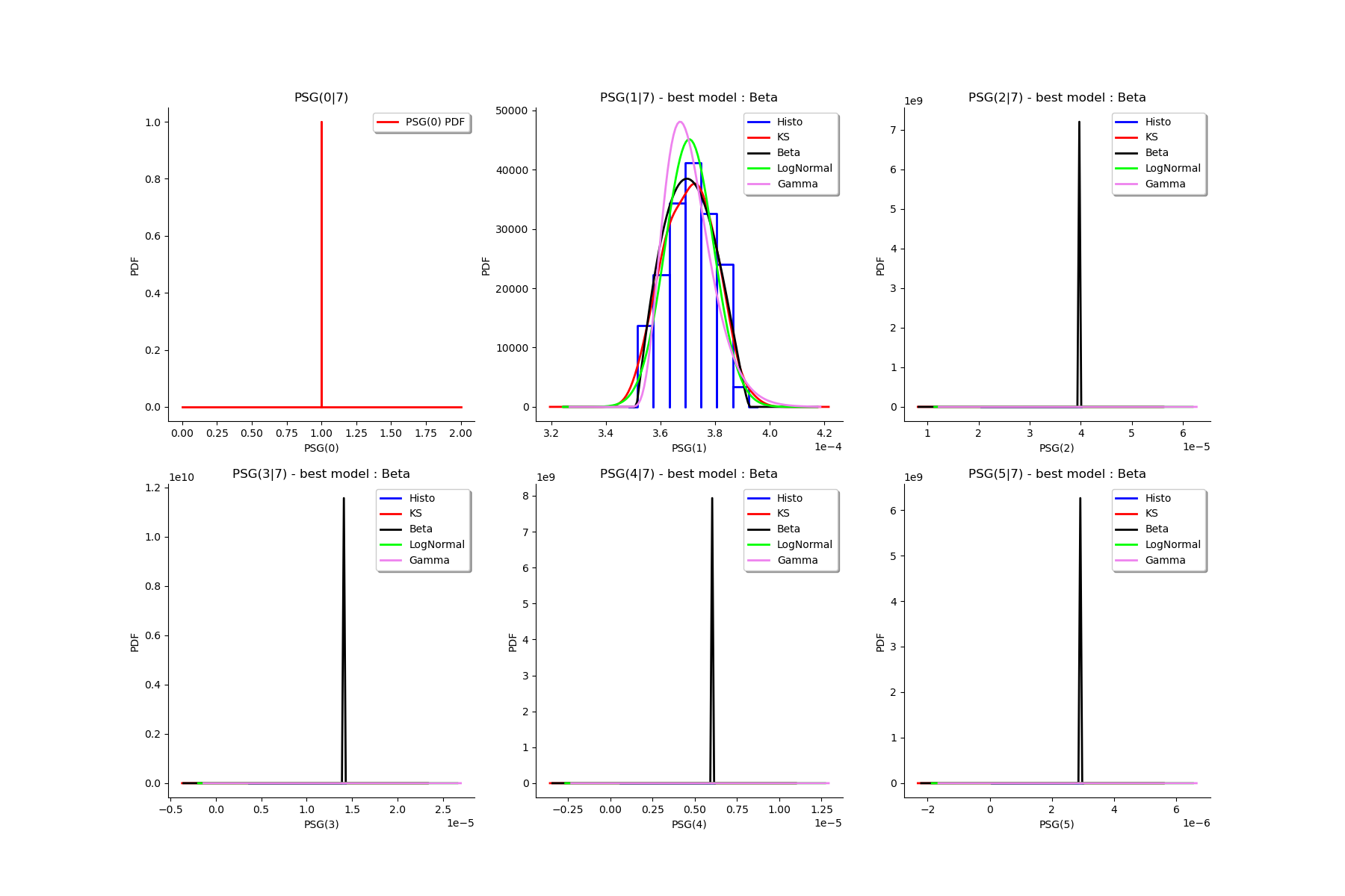
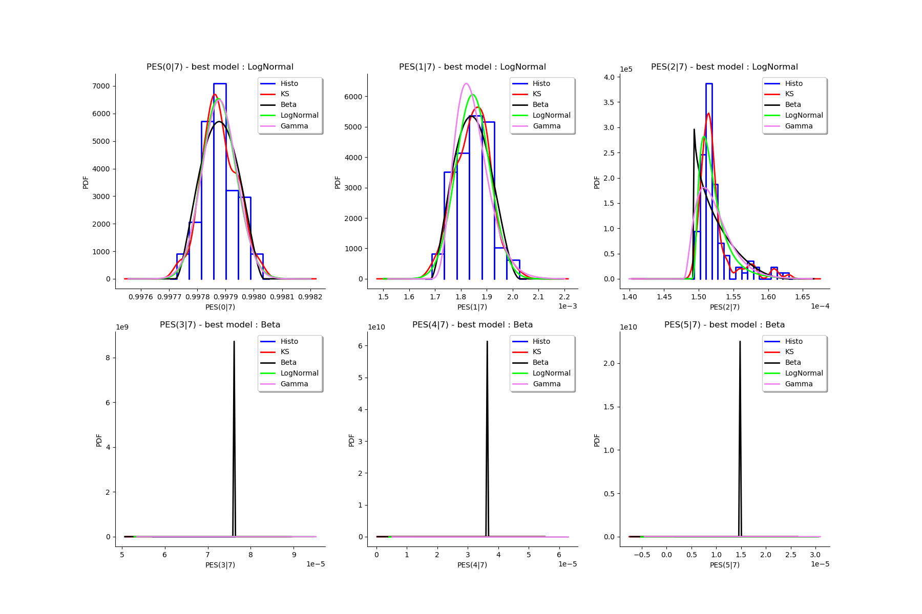
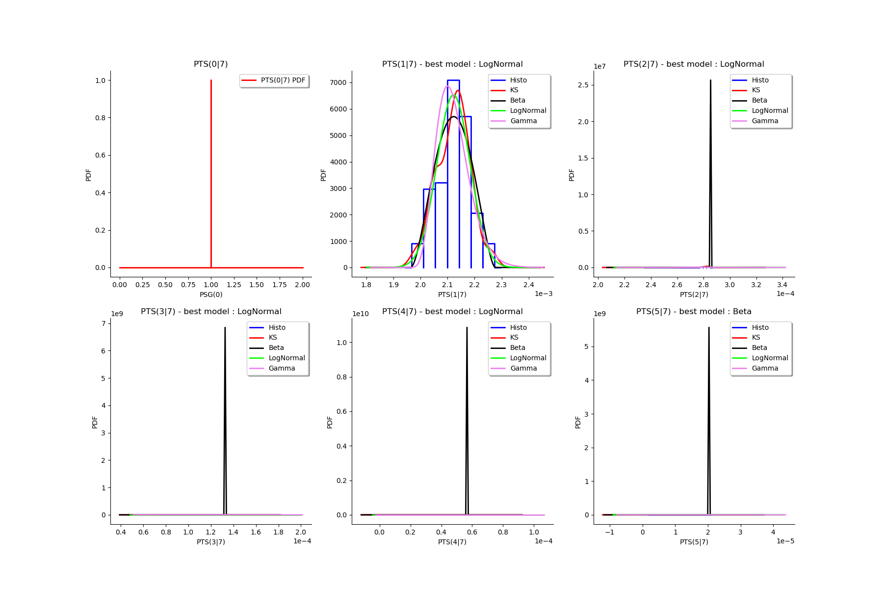
# We draw all the estimated distributions and the title gives the best model.

IC_PEG_ 0  =  [0.997776, 0.997987]
IC_PEG_ 1  =  [0.000247049, 0.00028004]
IC_PEG_ 2  =  [7.13113e-06, 7.53387e-06]
IC_PEG_ 3  =  [1.82805e-06, 2.17015e-06]
IC_PEG_ 4  =  [5.46603e-07, 1.03728e-06]
IC_PEG_ 5  =  [1.96105e-07, 7.00371e-07]
IC_PSG_ 0  =  [1, 1]
IC_PSG_ 1  =  [0.000354533, 0.000386447]
IC_PSG_ 2  =  [2.45992e-05, 3.956e-05]
IC_PSG_ 3  =  [5.5691e-06, 1.40086e-05]
IC_PSG_ 4  =  [1.4281e-06, 5.97618e-06]
IC_PSG_ 5  =  [4.06731e-07, 2.88145e-06]
IC_PES_ 0  =  [0.997776, 0.997987]
IC_PES_ 1  =  [0.00172934, 0.00196028]
IC_PES_ 2  =  [0.000149754, 0.000158211]
IC_PES_ 3  =  [6.39816e-05, 7.59626e-05]
IC_PES_ 4  =  [1.91311e-05, 3.6321e-05]
IC_PES_ 5  =  [4.1181e-06, 1.47119e-05]
IC_PTS_ 0  =  [1, 1]
IC_PTS_ 1  =  [0.00201273, 0.00222422]
IC_PTS_ 2  =  [0.000245838, 0.000284499]
IC_PTS_ 3  =  [8.78617e-05, 0.000132274]
IC_PTS_ 4  =  [2.38798e-05, 5.64708e-05]
IC_PTS_ 5  =  [4.74602e-06, 2.01807e-05]

gl = ot.GridLayout(2, 3)
for k in range(6):
    g = graphMargPEG_list[k]
    gl.setGraph(k//3, k%3, g)

# Deactivate grid to make matplotlib happy
gl = deactivateGrid(gl)
view = View(gl)
view.show()

gl = ot.GridLayout(2, 3)
for k in range(6):
    g = graphMargPSG_list[k]
    gl.setGraph(k//3, k%3, g)

# Deactivate grid to make matplotlib happy
gl = deactivateGrid(gl)
view = View(gl)
view.show()

gl = ot.GridLayout(2, 3)
for k in range(6):
    g = graphMargPES_list[k]
    gl.setGraph(k//3, k%3, g)

# Deactivate grid to make matplotlib happy
gl = deactivateGrid(gl)
view = View(gl)
view.show()

gl = ot.GridLayout(2, 3)
for k in range(6):
    g = graphMargPTS_list[k]
    gl.setGraph(k//3, k%3, g)

# Deactivate grid to make matplotlib happy
gl = deactivateGrid(gl)
view = View(gl)
view.show()

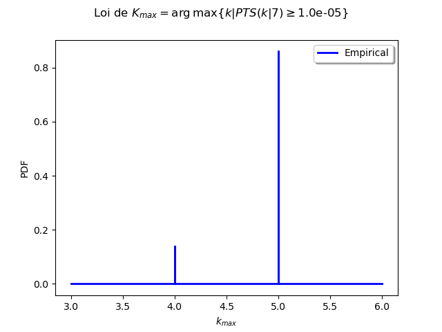
Analyse the minimal multiplicity which probability is greater than a given threshold

We fix p and we get the minimal multiplicity such that :

p = 1.0e-5
nameSeuil = '10M5'

kMax = myECLM.computeKMaxPTS(p)
print('kMax = ', kMax)

# Then we use the bootstrap sample of the Mankamo parameters to generate a sample of :math:`k_{max}`. We analyse the distribution of $k_{max}$: we estimate it with the empirical distribution and we derive a confidence interval of order :math:`90\%`.

kMax =  5

fileNameSampleParam = 'sampleParamFromMankamo_{}.csv'.format(Nbootstrap)
fileNameSampleKmax = 'sampleKmaxFromMankamo_{}_{}.csv'.format(Nbootstrap, nameSeuil)
# We use the parallelisation
parallel = True
gKmax = myECLM.computeAnalyseKMaxSample(p, fileNameSampleParam, fileNameSampleKmax, blocksize, parallel)

Confidence interval of level 90%: [ 4.0 ,  5.0 ]

gKmax.setGrid(False)
view = View(gKmax)
view.show()